
EXTRA-GALACTIC NEBULAE1
By EDWIN HUBBLE
[Transcriber’s Note: This etext was produced from
The Astrophysical Journal, Vol. LXIV, pp. 321-369, 1926.]
ABSTRACT
This contribution gives the results of a statistical investigation of 400 extra-galactic nebulae for which Holetschek has determined total visual magnitudes. The list is complete for the brighter nebulae in the northern sky and is representative to 12.5 mag. or fainter.
The classification employed is based on the forms of the photographic images. About 3 per cent are irregular, but the remaining nebulae fall into a sequence of type forms characterized by rotational symmetry about dominating nuclei. The sequence is composed of two sections, the elliptical nebulae and the spirals, which merge into each other.
Luminosity relations.—The distribution of magnitudes appears to be uniform throughout the sequence. For each type or stage in the sequence, the total magnitudes are related to the logarithms of the maximum diameters by the formula,  where C varies progressively from type to type, indicating a variation in diameter for a given magnitude or vice versa. By applying corrections to C, the nebulae can be reduced to a standard type and then a single formula expresses the relation for all nebulae from the Magellanic Clouds to the faintest that can be classified. When the minor diameter is used, the value of C is approximately constant throughout the entire sequence. The coefficient of log d corresponds with the inverse-square law, which suggests that the nebulae are all of the same order of absolute luminosity and that apparent magnitudes are measures of distance. This hypothesis is supported by similar results for the nuclear magnitudes and the magnitudes of the brightest stars involved, and by the small range in luminosities among nebulae whose distances are already known.
Distances and absolute dimensions.—The mean absolute visual magnitude, as derived from the nebulae whose distances are known, is –15.2. The statistical expression for the distance in parsecs is then  where mT is the total apparent magnitude. This leads to mean values for absolute dimensions at various stages in the sequence of types. Masses appear to be of the order of 2.6×10⁸ ☉.
Distribution and density of space.—To apparent magnitude about 16.7, corresponding to an exposure of one hour on fast plates with the 60-inch reflector, the numbers of nebulae to various limits of total magnitude vary directly with the volumes of space represented by the limits. This indicates an approximately uniform density of space, of the order of one nebula per 1017 cubic parsecs or 1.5×10⁻³¹ in C.G.S. units. The corresponding radius of curvature of the finite universe of general relativity is of the order of 2.7×10¹⁰ parsecs, or about 600 times the distance at which normal nebulae can be detected with the 100-inch reflector.
Recent studies have emphasized the fundamental nature of the division between galactic and extra-galactic nebulae. The relationship is not generic; it is rather that of the part to the whole. Galactic{2} nebulae are clouds of dust and gas mingled with the stars of a particular stellar system; extra-galactic nebulae, at least the most conspicuous of them, are now recognized as systems complete in themselves, and often incorporate clouds of galactic nebulosity as component parts of their organization. Definite evidence as to distances and dimensions is restricted to six systems, including the Magellanic Clouds. The similar nature of the countless fainter nebulae has been inferred from the general principle of the uniformity of nature.
The extra-galactic nebulae form a homogeneous group in which numbers increase rapidly with diminishing apparent size and luminosity. Four are visible to the naked eye;2 41 are found on the Harvard “Sky Map”;3 700 are on the Franklin-Adams plates;4 300,000 are estimated to be within the limits of an hour’s exposure with the 60-inch reflector.5 These data indicate a wide range in distance or in absolute dimensions. The present paper, to which is prefaced a general classification of nebulae, discusses such observational material as we now possess in an attempt to determine the relative importance of these two factors, distance and absolute dimensions, in their bearing on the appearance of extra-galactic nebulae.
The classification of these nebulae is based on structure, the individual members of a class differing only in apparent size and luminosity. It is found that for the nebulae in each class these characteristics are related in a manner which closely approximates the operation of the inverse-square law on comparable objects. The presumption is that dispersion in absolute dimensions is relatively unimportant, and hence that in a statistical sense the apparent dimensions represent relative distances. The relative distances can be reduced to absolute values with the aid of the nebulae whose distances are already known.
PART I. CLASSIFICATION OF NEBULAE
GENERAL CLASSIFICATION
The classification used in the present investigation is essentially the detailed formulation of a preliminary classification published in{3} a previous paper.6 It was developed in 1923, from a study of photographs of several thousand nebulae, including practically all the brighter objects and a thoroughly representative collection of the fainter ones.7 It is based primarily on the structural forms of photographic images, although the forms divide themselves naturally into two groups: those found in or near the Milky Way and those in moderate or high galactic latitudes. In so far as possible, the system is independent of the orientation of the objects in space. With minor changes in the original notation, the complete classification is as follows, although only the extra-galactic division is here discussed in detail:
CLASSIFICATION OF NEBULAE
| Symbol | Example | ||||||
|---|---|---|---|---|---|---|---|
| I. | Galactic nebulae: | ||||||
| A. | Planetaries | P | N.G.C. 7662 | ||||
| B. | Diffuse | D | |||||
| 1. | Predominantly luminous | DL | N.G.C. 6618 | ||||
| 2. | Predominantly obscure | DO | Barnard 92 | ||||
| 3. | Conspicuously mixed | DLO | N.G.C. 7023 | ||||
| II. | Extra-galactic nebulae: | ||||||
| A. | Regular: | ||||||
| 1. | Elliptical (n=1, 2, ..., 7 indicates the ellipticity of the image without the decimal point) |
En | N.G.C. 3379 E0 N.G.C. 221 E2 N.G.C. 4621 E5 N.G.C. 2117 E7{4} |
||||
| 2. | Spirals: | ||||||
| a) | Normal spirals | S | |||||
| (1) Early | Sa | N.G.C. 4594 | |||||
| (2) Intermediate | Sb | N.G.C. 2841 | |||||
| (3) Late | Sc | N.G.C. 5457 | |||||
| b) | Barred spirals | SB | |||||
| (1) Early | SBa | N.G.C. 2859 | |||||
| (2) Intermediate | SBb | N.G.C. 3351 | |||||
| (3) Late | SBc | N.G.C. 7479 | |||||
| B. | Irregular | Irr | N.G.C. 4449 | ||||
Extra-galactic nebulae too faint to be classified are designated by the symbol “Q.”
REGULAR NEBULAE
The characteristic feature of extra-galactic nebulae is rotational symmetry about dominating non-stellar nuclei. About 97 per cent of these nebulae are regular in the sense that they show this feature conspicuously. The regular nebulae fall into a progressive sequence ranging from globular masses of unresolved nebulosity to widely open spirals whose arms are swarming with stars. The sequence comprises two sections, elliptical nebulae and spirals, which merge into each other.
Although deliberate effort was made to find a descriptive classification which should be entirely independent of theoretical considerations, the results are almost identical with the path of development derived by Jeans8 from purely theoretical investigations. The agreement is very suggestive in view of the wide field covered by the data, and Jeans’s theory might have been used both to interpret the observations and to guide research. It should be borne in mind, however, that the basis of the classification is descriptive and entirely independent of any theory.
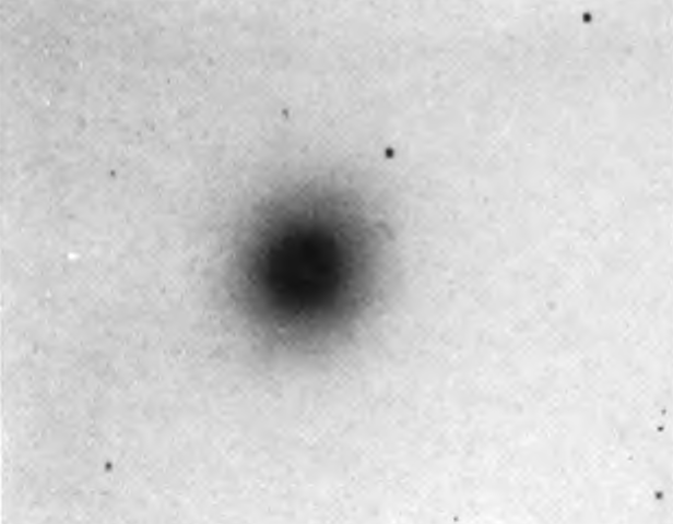
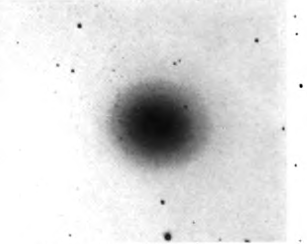
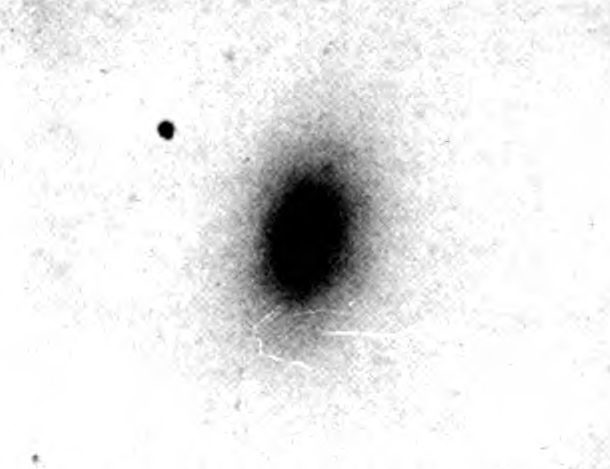
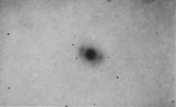
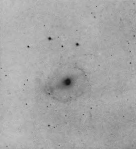
Elliptical nebulae.—These give images ranging from circular through flattening ellipses to a limiting lenticular figure in which the ratio of the axes is about 1 to 3 or 4. They show no evidence of resolution,9 and the only claim to structure is that the luminosity{5} fades smoothly from bright nuclei to indefinite edges. Diameters are functions of the nuclear brightness and the exposure times.
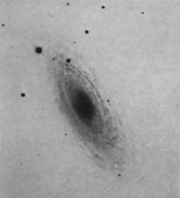
PLATE XII
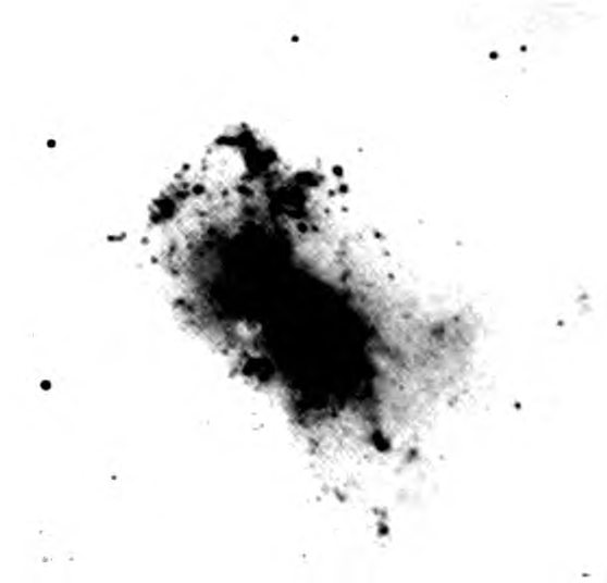
Elliptical and Irregular Nebulae
The only criterion available for further classification appears to be the degree of elongation. Elliptical nebulae have accordingly been designated by the symbol “E,” followed by a single figure, numerically equal to the ellipticity (a – b)/a with the decimal point omitted. The complete series is E0, E1, ..., E7, the last representing a definite limiting figure which marks the junction with the spirals.
The frequency distribution of ellipticities shows more round or nearly round images than can be accounted for by the random orientation of disk-shaped objects alone. It is presumed, therefore, that the images represent nebulae ranging from globular to lenticular, oriented at random. No simple method has yet been established for differentiating the actual from the projected figure of an individual object, although refined investigation furnishes a criterion in the relation between nuclear brightness and maximum diameters. For the present, however, it must be realized that any list of nebulae having a given apparent ellipticity will include a number of tilted objects having greater actual ellipticities. The statistical average will be too low, except for E7, and the error will increase with decreasing ellipticity.
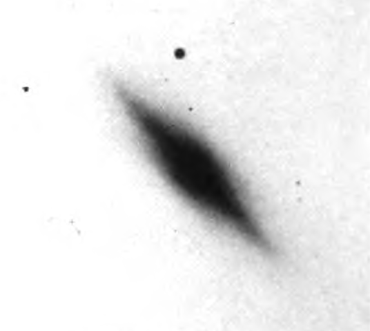
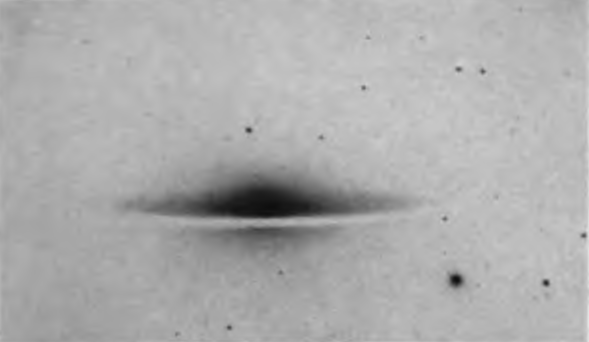
Normal spirals.—All regular nebulae with ellipticities greater than about E7 are spirals, and no spirals are known with ellipticities less than this limit. At this point in the sequence, however, ellipticity becomes insensitive as a criterion and is replaced by conspicuous structural features which now become available for classification. Of these, practically speaking, there are three which fix the position of an object in the sequence of forms: (1) relative size of the unresolved nuclear region; (2) extent to which the arms are unwound; (3) degree of resolution in the arms. The form most nearly related to the elliptical nebulae has a large nuclear region similar to E7, around which are closely coiled arms of unresolved nebulosity. Then follow objects in which the arms appear to build up at the expense of the nuclear regions and unwind as they grow; in the end, the arms are wide open and the nuclei inconspicuous. Early in the series the arms begin to break up into condensations, the resolution{6} commencing in the outer regions and working inward until in the final stages it reaches the nucleus itself. In the larger spirals where critical observations are possible, these condensations are found to be actual stars and groups of stars.
The structural transition is so smooth and continuous that the selection of division points for further classification is rather arbitrary. The ends of the series are unmistakable, however, and, in a general way, it is possible to differentiate a middle group. These three groups are designated by the non-committal letters “a,” “b,” and “c” attached to the spiral symbols “S,” and, with reference to their position in the sequence, are called “early,” “intermediate,” and “late” types.10 A more precise subdivision, on a decimal scale for example, is not justified in the present state of our knowledge.
In the early types, the group Sa, most of the nebulosity is in the nuclear region and the arms are closely coiled and unresolved. N.G.C. 3368 and 4274 are among the latest of this group.
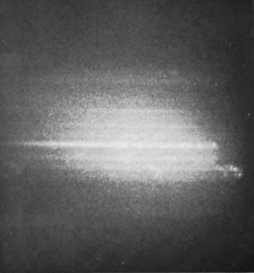
The intermediate group, Sb, includes objects having relatively large nuclear regions and thin rather open arms, as in M 81, or a smaller nuclear region with closely coiled arms, as in M 94. These two nebulae represent the lateral extension of the sequence in the intermediate section. The extension along the sequence is approximately represented by N.G.C. 4826, among the earliest of the Sb, and N.G.C. 3556 and 7331, which are among the latest. The resolution in the arms is seldom conspicuous, although in M 31, a typical Sb, it is very pronounced in the outer portions.
PLATE XIII
Normal and Barred Spirals
{7}
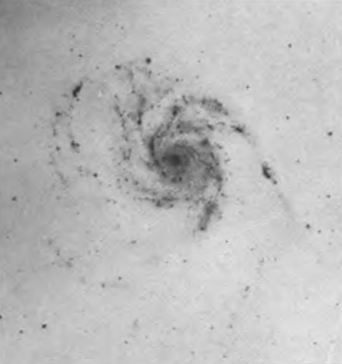
The characteristics of the late types, the group Sc, are more definite—an inconspicuous nucleus and highly resolved arms. Individual stars cannot be seen in the smaller nebulae of this group, but knots are conspicuous, which, in larger objects, are known to be groups and clusters of stars. The extent to which the arms are opened varies from M 33 to M 101, both typical Sc nebulae.
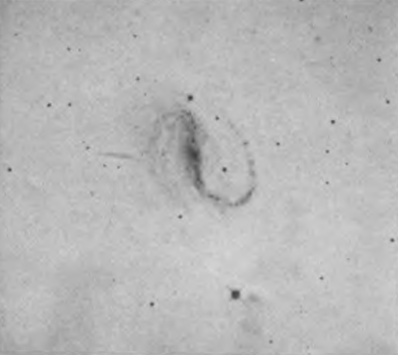
Barred spirals.—In the normal spiral the arms emerge from two opposite points on the periphery of the nuclear region. There is, however, a smaller group, containing about 20 per cent of all spirals, in which a bar of nebulosity extends diametrically across the nucleus. In these spirals, the arms spring abruptly from the ends of this bar. These nebulae also form a sequence, which parallels that of the normal spirals, the arms apparently unwind, the nuclei dwindle, the condensations form and work inward.
H. D. Curtis11 first called attention to these nebulae when he described several in the intermediate stages of the series and called them φ-type spirals. The bar, however, never extends beyond the inner spiral arms, and the structure, especially in the early portion of the sequence, is more accurately represented by the Greek letter θ. From a dynamical point of view, the distinction has considerable significance. Since Greek letters are inconvenient for cataloguing purposes, the English term, “barred spiral,” is proposed, which can be contracted to the symbol “SB.”
The SB series, like that of the normal spirals, is divided into three roughly equal sections, distinguished by the appended letters “a,” “b,” and “c.” The criteria on which the division is based are similar in general to those used in the classification of the normal spirals. In the earliest forms, SBa, the arms are not differentiated, and the pattern is that of a circle crossed by a bar, or, as has been mentioned, that of the Greek letter θ. When the bar is oriented nearly in the line of sight, it appears foreshortened as a bright and definite minor axis of the elongated nebular image. Such curious forms as the images of N.G.C. 1023 and 3384 are explained in this manner. The latest group, SBc, is represented by the S-shaped spirals such as N.G.C. 7479.
{8}
IRREGULAR NEBULAE
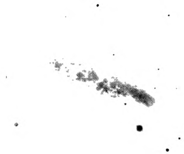
About 3 per cent of the extra-galactic nebulae lack both dominating nuclei and rotational symmetry. These form a distinct class which can be termed “irregular.” The Magellanic Clouds are the most conspicuous examples, and, indeed, are the nearest of all the extra-galactic nebulae. N.G.C. 6822, a curiously faithful miniature of the Clouds, serves to bridge the gap between them and the smaller objects, such as N.G.C. 4214 and 4449. In these latter, a few individual stars emerge from an unresolved background, and occasional isolated spots give the emission spectrum characteristic of diffuse nebulosity in the galactic system, in the Clouds, and in N.G.C. 682212 These features are found in other irregular nebulae as well, notably in N.G.C. 1156 and 4656, and are just those to be expected in systems similar to the Clouds but situated at increasingly greater distances.
The system outlined above is primarily for the formal classification of photographic images obtained with large reflectors and portrait lenses. For each instrument, however, there is a limiting size and luminosity below which it is impossible to classify with any confidence. Except in rare instances, these small nebulae are extra-galactic, and their numbers, brightness, dimensions, and distribution are amenable to statistical investigation. For cataloguing purposes, they require a designating symbol, and the letter “Q” is suggested as convenient and not too widely used with other significations.
PLATE XIV
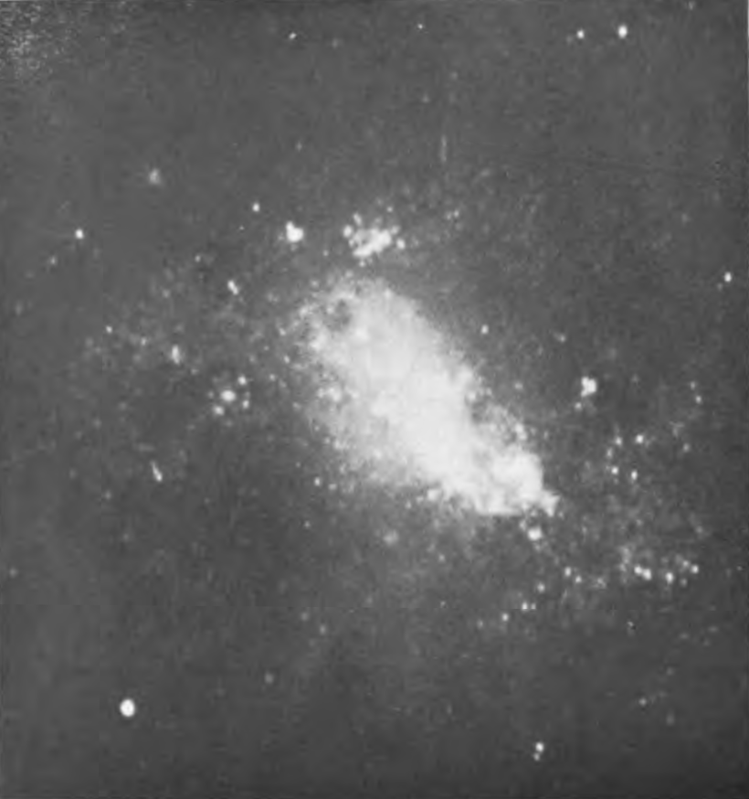
Irregular Nebula N.G.C. 4214
PART II. STATISTICAL STUDY OF EXTRA-GALACTIC NEBULAE
THE DATA
The most homogeneous list of nebulae for statistical study is that compiled by Hardcastle13 containing all nebulae found on the Franklin-Adams charts. These are uniform exposures of two hours on fast plates made with a Cooke astrographic lens of 10-inch aperture and 45-inch focal length. The scale is 1 mm = 3′. The entire sky is covered,{9} but since the plates are centered about 15° apart and the definition decreases very appreciably with distance from the optical axis, the material is not strictly homogeneous. Moreover, the published list suffers from the usual errors attendant on routine cataloguing; for instance, four conspicuous Messier nebulae, M 60, M 87, M 94, and M 101, are missing. In general, however, the list is thoroughly representative down to about the thirteenth photographic magnitude and very few conspicuous objects are overlooked. It plays the role of a standard with which other catalogues of the brighter nebulae may be compared for completeness, and numbers in limited areas may be extended to the entire sky.
When known galactic nebulae, clusters, and the objects in the Magellanic Clouds are weeded out, the remaining 700 nebulae may be treated as extra-galactic. Very few can be classified from the Franklin-Adams plates; for this purpose photographs on a much larger scale are required. Until further data on the individual objects are available, Hardcastle’s list can be used only for the study of distribution over the sky. This shows the well-known features—the greater density in the northern galactic hemisphere, the concentration in Virgo, and the restriction of the very large nebulae to the southern galactic hemisphere.
Fortunately, numerical data do exist in the form of total visual magnitudes for many of the nebulae in the northern sky. These determinations were made by Holetschek,14 who attempted to observe all nebulae within reach of his 6-inch refractor. He later restricted his program; but the final list is reasonably complete for the more conspicuous nebulae north of declination –10°, and is representative down to visual magnitude about 12.5. Out of 417 extra-galactic nebulae in Holetschek’s list, 408 are north of –10°, as compared with 400 in Hardcastle’s. The two lists agree very well for the brighter objects, but diverge more and more with decreasing luminosity. At the twelfth magnitude about half of Holetschek’s nebulae are included by Hardcastle. Since the two lists compare favorably in completeness over so large a region of the sky, Holetschek’s may be chosen as the basis for a statistical study and advantage taken of the valuable numerical data on total luminosities.
{10}
Hopmann15 has revised the scale of magnitudes by photometric measures of the comparison stars used by Holetschek. New magnitudes were thus obtained for 85 individual nebulae and from these were derived mean correction tables applicable to the entire list. The revised magnitudes are used throughout the following discussion. Hopmann’s corrections extend to about 12.0 mag., and have been extrapolated on the assumption that they are constant for the fainter magnitudes. The errors involved are unimportant in view of selective effects which must be present among the observed objects near the limit of visibility.
The nebulae were classified and their diameters measured from photographs of about 300 of them taken with the 60-inch and 100-inch reflectors at Mount Wilson. Most of the others are included in the great collection of nebular photographs at Mount Hamilton, which have been described by Curtis;16 and, through the courtesy of the Director of the Lick Observatory, it has been possible to confirm the classification inferred from the published description by actual inspection of the original negatives.
Types, diameters, and total visual magnitudes are thus available for some 400 of the nebulae in Holetschek’s list. The few unclassified objects are all fainter than 12.5 mag. The data are listed in Tables I–IV, in which the N.G.C. numbers, the total magnitudes, and the logarithms of the maximum diameters in minutes of arc are given for each type separately. A summary is given in Table V, in which the relative frequencies and the mean magnitudes of the various types will be found.
RELATIVE LUMINOSITIES OF THE VARIOUS TYPES
The frequency distribution of magnitudes for all types together and for the elliptical nebulae and the spirals separately is shown in Table VI and Figure 1. With the exception of the two outstanding spirals, M 31 and M 33, the apparent luminosities are about uniformly distributed among the different types. The relative numbers of the elliptical nebulae as compared with the spirals decrease somewhat with decreasing luminosity, but this is very probably an effect{11} of selection. The elliptical nebulae are more compact than the spirals and become more stellar with decreasing luminosity. For this reason some of the fainter nebulae are missed when small-scale instruments are used, although the same luminosity spread over a larger area would still be easily detected. The effect is very pronounced on photographic plates. It accounts also for the slightly brighter mean magnitude of the elliptical nebulae as compared with the spirals in Table V.
TABLE I
Elliptical Nebulae
| N.G.C. | mT | log d |
|---|---|---|
| E0 (17) | ||
| 404 | 11.1 | +0.11 |
| 474 | 12.6 | – .40 |
| 1407 | 10.9 | .15 |
| 3348 | 11.8 | – .15 |
| 3379* | 9.4 | + .30 |
| 4283 | 12.2 | – .52 |
| 4486* | 9.7 | + .30 |
| 4494* | 10.1 | – .15 |
| 4552* | 9.9 | + .23 |
| 4589 | 11.4 | – .30 |
| 4648 | 12.3 | .52 |
| 5044 | 11.8 | .30 |
| 5216 | 13.3 | .70 |
| 5273 | 12.1 | .52 |
| 5557 | 12.3 | .40 |
| 5812 | 12.0 | – .40 |
| 5846 | 10.9 | 0.0 |
| Mean | 11.40 | –0.204 |
| E1 (13) | ||
| 467 | 13.0 | –0.70 |
| 596 | 11.8 | .22 |
| 1400 | 11.1 | .22 |
| 2880 | 12.0 | .52 |
| 3226 | 12.0 | .10 |
| 3962 | 11.8 | – .30 |
| 4278* | 10.8 | .0 |
| 4374* | 9.9 | + .08 |
| 4472 | 8.8 | + .30 |
| 4478 | 11.5 | – .10 |
| 4636 | 10.9 | + .08 |
| 5813 | 12.6 | – .30 |
| 7626 | 12.3 | –0.30 |
| Mean | 11.43 | –0.177 |
| E2 (14) | ||
| 221* | 8.8 | +0.42 |
| 1453 | 11.9 | – .10 |
| 2672 | 12.8 | – .40 |
| 3193 | 12.1 | 0.0 |
| 3599 | 12.0 | –0.30 |
| 3608 | 11.6 | .22 |
| 3640 | 11.1 | – .05 |
| 4261 | 11.1 | + .20 |
| 4291 | 12.3 | – .52 |
| 4377 | 11.9 | – .05 |
| 4406* | 10.0 | + .30 |
| 4476 | 12.8 | – .30 |
| 4649* | 9.5 | + .30 |
| 5127 | 13.3 | –0.52 |
| Mean | 11.52 | –0.088 |
| E3 (10) | ||
| 1052 | 11.8 | –0.15 |
| 1600 | 12.7 | + .17 |
| 3222 | 13.3 | – .15 |
| 4319 | 12.8 | – .52 |
| 4365 | 11.4 | + .04 |
| 4386 | 12.3 | – .52 |
| 5322* | 9.6 | + .15 |
| 5982 | 11.4 | .0 |
| 7562 | 12.8 | – .22 |
| 7619 | 11.8 | – .15 |
| Mean | 11.99 | –0.133 |
| E4 (13) | ||
| 584 | 10.9 | +0.30 |
| 1700 | 12.5 | – .10 |
| 2974 | 11.8 | .15 |
| 3605 | 12.5 | – .52 |
| 3610 | 11.8 | + .15 |
| 3894 | 12.8 | – .05 |
| 4125* | 10.3 | + .30 |
| 4378 | 12.1 | – .15 |
| 4382* | 10.0 | + .48 |
| 4551 | 12.8 | + .04 |
| 4742 | 12.3 | .0 |
| 5576 | 12.3 | – .15 |
| 7454 | 13.3 | 0.0 |
| Mean | 11.95 | –0.011 |
| E5 (6){12} | ||
| 720 | 10.9 | + .11 |
| 2693 | 12.3 | – .15 |
| 3377 | 10.9 | + .17 |
| 4473 | 10.3 | .11 |
| 4621* | 10.0 | + .30 |
| 4660 | 11.4 | 0.0 |
| Mean | 10.97 | +0.090 |
| E6 (7) | ||
| 821 | 11.8 | 0.0 |
| 2768 | 10.7 | + .18 |
| 3613 | 11.8 | .25 |
| 4179 | 11.8 | .34 |
| 4435* | 10.5 | .11 |
| 4546* | 10.3 | .18 |
| 4697* | 9.6 | +0.48 |
| Mean | 10.93 | +0.220 |
| E7 (5) | ||
| 3115* | 9.5 | +0.60 |
| 4111 | 10.1 | .54 |
| 4270 | 12.1 | .0 |
| 4570 | 11.1 | .38 |
| 5308 | 12.3 | +0.28 |
| Mean | 11.02 | +0.360 |
| Peculiar (8) | ||
| 185 | 12.3 | +0.48 |
| 205* | 9.3 | .90 |
| 524† | 11.9 | .41 |
| 3607† | 9.9 | .11 |
| 3998† | 12.1 | + .23 |
| 4459‡ | 11.3 | – .22 |
| 5485‡ | 12.3 | .05 |
| 5739 | 13.3 | –0.40 |
The various types are homogeneously distributed over the sky, their spectra are similar, and the radial velocities are of the same general order. These facts, together with the equality of the mean magnitudes and the uniform frequency distribution of magnitudes, are consistent with the hypothesis that the distances and absolute luminosities as well are of the same order for the different types. This is an assumption of considerable importance, but unfortunately it cannot yet be subjected to positive and definite tests. None of the individual similarities necessarily implies the adopted interpretation, but the totality of them, together with the intimate series relations{13} among the types, which will be discussed later, suggests it as the most reasonable working hypothesis, at least until inconsistencies should appear.
TABLE II
Barred Spirals
| N.G.C. | mT | log d |
|---|---|---|
| SBa (26) | ||
| 936 | 11.1 | +0.48 |
| 1023* | 10.2 | .78 |
| 2732 | 12.3 | .11 |
| 2781 | 12.3 | .11 |
| 2787 | 11.4 | .36 |
| 2859 | 11.1 | .28 |
| 2950 | 11.6 | .15 |
| 3384* | 10.7 | .48 |
| 3412* | 11.2 | + .40 |
| 3418 | 13.1 | .0 |
| 3458 | 12.8 | – .22 |
| 3945 | 11.5 | + .20 |
| 4026 | 11.1 | .48 |
| 4203 | 11.1 | .36 |
| 4346 | 12.0 | .20 |
| 4371 | 12.0 | .18 |
| 4421 | 12.8 | .17 |
| 4442 | 10.9 | .50 |
| 4477 | 10.9 | .40 |
| 4596 | 12.0 | .25 |
| 4643 | 11.1 | .26 |
| 4754 | 10.9 | .48 |
| 5473 | 12.0 | + .08 |
| 5574 | 13.0 | – .05 |
| 5689 | 12.0 | + .30 |
| 5701 | 12.3 | +0.17 |
| Mean | 11.66 | +0.267 |
| SBb (16) | ||
| 1022 | 11.8 | +0.04 |
| 2650 | 12.8 | .0 |
| 3351* | 11.4 | + .48 |
| 3400 | 12.5 | – .10 |
| 3414 | 11.5 | + .26 |
| 3504 | 11.4 | .30 |
| 3718 | 11.8 | +0.48 |
| 4102 | 12.0 | +0.36 |
| 4245 | 11.1 | .15 |
| 4394 | 11.5 | .60 |
| 4548 | 11.1 | .60 |
| 4699* | 10.0 | .57 |
| 4725* | 9.2 | .70 |
| 5218 | 12.8 | .25 |
| 5566 | 11.1 | .20 |
| 7723 | 11.8 | +0.18 |
| Mean | 11.48 | +0.317 |
| SBc (15) | ||
| 613 | 10.6 | +0.60 |
| 779 | 12.1 | .48 |
| 3206 | 13.3 | .45 |
| 3344 | 11.4 | .60 |
| 3346 | 12.3 | .40 |
| 3625 | 13.3 | .0 |
| 3686 | 12.0 | .30 |
| 3769 | 12.8 | .43 |
| 3953 | 11.1 | .74 |
| 3992 | 11.5 | .85 |
| 4303* | 10.6 | .78 |
| 4579* | 9.7 | .45 |
| 5383 | 12.6 | .40 |
| 5921 | 12.8 | .70 |
| 7479 | 12.1 | +0.48 |
| Mean | 11.87 | +0.509 |
| Peculiar (2) | ||
| 2782 | 12.3 | +0.26 |
| 4314 | 11.1 | +0.34 |
{14}
TABLE III
Normal Spirals
| N.G.C. | mT | log d |
|---|---|---|
| Sa (49) | ||
| 488 | 11.8 | +0.48 |
| 676 | 13.3 | .30 |
| 1332 | 10.9 | .43 |
| 2655 | 11.1 | .60 |
| 2681 | 10.7 | .48 |
| 2775 | 10.9 | .32 |
| 2811 | 12.3 | .28 |
| 2855 | 12.8 | .11 |
| 3169§ | 12.3 | .60 |
| 3245 | 11.8 | .30 |
| 3301 | 12.4 | .15 |
| 3368* | 10.0 | .85 |
| 3516 | 12.1 | .20 |
| 3619 | 12.3 | .0 |
| 3626* | 11.3 | .28 |
| 3665 | 12.0 | .0 |
| 3682 | 12.1 | .08 |
| 3898 | 12.0 | .43 |
| 3941 | 10.3 | .30 |
| 4036 | 10.9 | .60 |
| 4138 | 12.1 | .20 |
| 4143 | 11.3 | .11 |
| 4150 | 12.0 | .11 |
| 4251 | 10.4 | .26 |
| 4268 | 12.8 | .0 |
| 4274 | 11.1 | +0.54 |
| 4281 | 11.5 | +0.18 |
| 4429 | 11.5 | .48 |
| 4452 | 12.6 | .15 |
| 4526 | 11.1 | .70 |
| 4550 | 12.1 | .43 |
| 4570 | 11.1 | .38 |
| 4594 | 9.1 | .85 |
| 4665 | 11.8 | + .08 |
| 4684 | 12.2 | – .22 |
| 4698 | 11.9 | + .43 |
| 4710 | 11.8 | .54 |
| 4762 | 11.5 | .57 |
| 4866 | 12.0 | .50 |
| 4958 | 11.4 | .60 |
| 5377 | 11.8 | .48 |
| 5389 | 12.5 | .25 |
| 5422 | 12.1 | + .40 |
| 5631 | 12.0 | – .05 |
| 5866* | 11.7 | + .48 |
| 7013 | 12.8 | .08 |
| 7457 | 12.8 | .30 |
| 7727 | 11.3 | .43 |
| 7814* | 11.4 | +0.48 |
| Mean | 11.69 | +0.333 |
| Sb (70) | ||
| 224 | 5.0 | +2.25 |
| 672 | 12.8 | 0.54 |
| 772 | 11.1 | .70 |
| 949 | 13.3 | .0 |
| 955 | 12.9 | .40 |
| 1068 | 9.1 | .40 |
| 1309 | 12.0 | .15 |
| 2639 | 12.2 | .0 |
| 2715 | 12.5 | .40 |
| 2748 | 12.0 | .32 |
| 2841* | 9.4 | .78 |
| 2985 | 11.4 | 0.48 |
| 3031* | 8.3 | +1.20 |
| 3182 | 12.9 | –0.22 |
| 3190 | 11.9 | + .48 |
| 3227 | 12.0 | .48 |
| 3277 | 12.6 | .0 |
| 3310 | 10.4 | + .18 |
| 3380 | 12.1 | – .05 |
| 3489* | 11.2 | +0.40 |
| 3556 | 11.1 | +0.90 |
| 3593 | 11.9 | .60 |
| 3623* | 9.9 | .90 |
| 3627* | 9.1 | 0.90 |
| 3628§ | 11.4 | +1.08 |
| 3632 | 13.3 | –0.10 |
| 3675 | 11.4 | + .48 |
| 3681 | 13.0 | .0 |
| 3684 | 13.0 | + .08 |
| 3895 | 13.3 | – .05 |
| 3900 | 12.1 | + .25 |
| 3938 | 12.1 | .65 |
| 4020 | 12.3 | .17 |
| 4030 | 11.1 | .30 |
| 4051* | 11.9 | .60 |
| 4085 | 12.5 | .36 |
| 4151 | 12.0 | .40 |
| 4192 | 10.9 | .90 |
| 4216* | 10.8 | 0.85 |
| 4244§ | 12.3 | +1.11{15} |
| 4258* | 8.7 | +1.30 |
| 4273 | 11.8 | 0.20 |
| 4438* | 10.3 | .54 |
| 4448 | 11.8 | .48 |
| 4450 | 10.6 | + .57 |
| 4451 | 12.8 | – .15 |
| 4500 | 12.8 | +0.17 |
| 4565*§ | 11.0 | 1.17 |
| 4736* | 8.4 | 0.70 |
| 4750 | 11.8 | .26 |
| 4800 | 11.8 | .04 |
| 4814 | 12.7 | .56 |
| 4826 | 9.0 | .90 |
| 5055* | 9.6 | .90 |
| 5376 | 12.8 | + .17 |
| 5379 | 12.9 | –0.05 |
| 5394 | 13.3 | +0.17 |
| 5633 | 13.0 | – .10 |
| 5713 | 12.3 | + .32 |
| 5740 | 12.3 | .48 |
| 5746 | 10.4 | .87 |
| 5750 | 12.8 | .15 |
| 5772 | 12.0 | .25 |
| 5806 | 12.3 | .30 |
| 5985 | 12.0 | .60 |
| 6207 | 11.8 | .30 |
| 6643 | 11.9 | .48 |
| 7331* | 10.4 | .95 |
| 7541 | 12.7 | .41 |
| 7606 | 12.0 | +0.78 |
| Mean | 11.55 | +0.471 |
| Sc (115) | ||
| 157 | 11.4 | +0.40 |
| 253 | 9.3 | 1.34 |
| 278 | 12.0 | 0.08 |
| 470 | 13.1 | 0.20 |
| 598 | 7.0 | 1.78 |
| 615 | 12.3 | 0.43 |
| 628* | 10.6 | .90 |
| 908 | 11.9 | .60 |
| 1084 | 11.4 | .34 |
| 1087 | 12.1 | .36 |
| 1637 | 12.6 | .48 |
| 2339 | 13.1 | 0.28 |
| 2403* | 8.7 | 1.20 |
| 2532 | 13.3 | 0.17 |
| 2683 | 9.9 | 1.00 |
| 2712 | 12.3 | 0.20 |
| 2742 | 11.8 | .40 |
| 2776 | 12.3 | 0.34 |
| 2903* | 9.1 | 1.04 |
| 2964 | 11.6 | .40 |
| 2976 | 12.0 | .50 |
| 3003§ | 13.3 | .78 |
| 3021 | 12.3 | .11 |
| 3079§ | 12.0 | .90 |
| 3147 | 11.4 | .30 |
| 3166 | 12.0 | .0 |
| 3184 | 12.7 | .78 |
| 3198 | 13.0 | .95 |
| 3254 | 12.8 | .60 |
| 3294 | 12.0 | .48 |
| 3389 | 13.1 | +0.30 |
| 3395 | 12.6 | +0.11 |
| 3396 | 13.3 | – .10 |
| 3430 | 12.6 | + .49 |
| 3432 | 12.0 | .79 |
| 3437 | 12.4 | .28 |
| 3445 | 13.1 | .08 |
| 3448 | 12.3 | .26 |
| 3486 | 11.8 | .58 |
| 3488 | 12.8 | .25 |
| 3512 | 12.3 | .0 |
| 3521* | 10.1 | .65 |
| 3549 | 13.3 | .43 |
| 3596 | 13.3 | .60 |
| 3631 | 11.8 | .66 |
| 3642 | 12.0 | .73 |
| 3655 | 11.9 | .04 |
| 3666 | 11.8 | .54 |
| 3672 | 13.0 | .54 |
| 3683 | 12.0 | .15 |
| 3780 | 13.0 | .40 |
| 3810 | 11.3 | .62 |
| 3813 | 12.3 | .32 |
| 3877 | 11.8 | .64 |
| 3887 | 12.3 | .40 |
| 3893 | 11.8 | .61 |
| 3949 | 11.8 | .34 |
| 3982 | 12.1 | .36 |
| 4013 | 13.3 | .60 |
| 4041 | 11.4 | .30 |
| 4062 | 12.6 | .48 |
| 4088 | 11.5 | .+0.72{16} |
| 4096 | 12.3 | +0.78 |
| 4100 | 12.3 | .60 |
| 4145 | 12.3 | .70 |
| 4157§ | 12.3 | .77 |
| 4212 | 12.3 | .30 |
| 4220 | 12.1 | 0.40 |
| 4236 | 12.8 | 1.04 |
| 4254 | 10.4 | 0.65 |
| 4321* | 10.5 | .70 |
| 4414 | 10.1 | .48 |
| 4419 | 11.8 | .36 |
| 4460 | 12.1 | .20 |
| 4490* | 10.2 | .60 |
| 4501* | 10.5 | .70 |
| 4504 | 12.1 | 0.48 |
| 4517§ | 12.5 | 1.00 |
| 4536§ | 12.3 | 0.85 |
| 4559 | 10.7 | .90 |
| 4569* | 10.9 | .65 |
| 4580 | 12.3 | .15 |
| 4605 | 9.9 | 0.48 |
| 4631* | 9.5 | 1.08 |
| 4632 | 13.1 | 0.50 |
| 4666 | 12.0 | .60 |
| 4713 | 12.3 | .38 |
| 4781 | 11.8 | .48 |
| 4793 | 12.4 | .20 |
| 4808 | 12.6 | +0.34 |
| 4995 | 11.8 | +0.36 |
| 5005* | 11.1 | .70 |
| 5012 | 11.9 | .43 |
| 5033* | 11.8 | 0.78 |
| 5194* | 7.4 | 1.08 |
| 5204 | 12.8 | 0.59 |
| 5236 | 10.4 | 1.00 |
| 5247 | 13.3 | 0.70 |
| 5248 | 11.5 | .50 |
| 5290 | 12.5 | .48 |
| 5297 | 12.6 | .60 |
| 5364 | 13.3 | .60 |
| 5395 | 12.8 | 0.30 |
| 5457 | 9.9 | 1.34 |
| 5474 | 12.0 | 0.60 |
| 5585 | 12.3 | .60 |
| 5676 | 11.8 | .48 |
| 5678 | 11.8 | .41 |
| 5832 | 13.1 | 0.56 |
| 5907§ | 11.9 | 1.04 |
| 6181 | 12.5 | 0.30 |
| 6217 | 12.1 | .25 |
| 6503 | 9.9 | .70 |
| 7448 | 11.8 | + .30 |
| 7671 | 13.3 | – .15 |
| Mean | 11.75 | +0.537 |
| Peculiar Spirals (Unclassified) | ||
| 972 | 13.3 | +0.17 |
| 2537 | 13.3 | .0 |
| 4900 | 11.8 | +0.23 |
RELATION BETWEEN LUMINOSITIES AND DIAMETERS
Among the nebulae of each separate type are found linear correlations between total magnitudes and logarithms of diameters. These are shown in Figures 2–5 for the beginning, middle, and end of the sequence of types and also for the irregular nebulae. In Figures 2 and 3 adjacent types have been grouped in order to increase the material, and in Figure 5 the Magellanic Clouds have been added to increase the range.
The correlations can be expressed in the form
 |
(1) |
where K is constant from type to type, but C varies progressively throughout the sequence. The value of K cannot be accurately determined{17} from the scattered data for any particular type, but, within the limits of uncertainty, it approximates the round number 5.0, the value which is represented by the lines in Figures 2–5.
When K is known, the value of C can be computed from the mean magnitude and the logarithm of the diameter for each type. This amounts to reading from the curves the magnitudes corresponding to a diameter of one minute of arc, but avoids the uncertainty of establishing the curves where the data are limited.
TABLE IV
Irregular Nebulae
| N.G.C. | mT | log d |
|---|---|---|
| 2968 | 12.6 | +0.08 |
| 3034* | 9.0 | .85 |
| 3077 | 11.4 | .48 |
| 3729 | 11.8 | .17 |
| 4214* | 11.3 | .90 |
| 4449* | 9.5 | .65 |
| 4618 | 12.3 | +0.40 |
| 4656§ | 11.5 | +1.30 |
| 4753 | 11.4 | +0.43 |
| 5144 | 12.8 | – .30 |
| 5363 | 11.1 | +0.20 |
| Mean | 11.34 | +0.469 |
NOTES TO TABLES I–IV
* Magnitude from Hopmann.
† N.G.C. 524 and 3998 are late elliptical nebulae in which the equatorial planes are perpendicular to the line of sight. They might be included with the E6 or E7 nebulae.
§ Absorption very conspicuous.
‡ N.G.C. 3607, 4459, and 5485 appear to be elliptical nebulae with narrow bands of absorption between the nuclei and the peripheries.
The progressive change in the value of C throughout the sequence may be expressed as a variation either in the magnitude for a given diameter or in the diameter for a given magnitude. Both effects are listed in Table VII and are illustrated in Figure 6, in which magnitudes and diameters thus found are plotted against types. With the exception of the later elliptical nebulae, for which the data are wholly inadequate for reliable determinations, the points fall on smooth curves. In the region of the earlier elliptical nebulae, the curves should be somewhat steeper in order to allow for objects of greater ellipticities which are probably included.
REDUCTION OF NEBULAE TO A STANDARD TYPE
The slope, K, in the formula relating magnitudes with diameters, appears to be closely similar for the various types, but accurate determinations{18} are restricted by the limited and scattered nature of the data for each type separately. With a knowledge of the parameter C, however, it is possible to reduce all the material to a standard{19} type and hence to determine the value of K from the totality of the data. The mean of E7, SBa, and Sa was chosen for the purpose, as representing a hypothetical transition-point between the elliptical nebulae and the spirals, and was designated by the symbol “S0.” The corresponding value of C, in round numbers, is 13.0. Corrections were applied to the logarithms of the diameters of the nebulae of each observed class, amounting to  where C is the observed value for a particular class.17 When the values of C are read from the smooth curve in Figure 6, these corrections are as shown in Table VIII.
TABLE V
Frequency Distribution of Types
| Type | Number | Percentage | Mean Mag. |
|---|---|---|---|
| Elliptical Nebulae | |||
| E0 | 17 | 18 | 11.40 |
| 1 | 13 | 14 | 11.43 |
| 2 | 14 | 15 | 11.52 |
| 3 | 10 | 11 | 11.99 |
| 4 | 13 | 14 | 11.95 |
| 5 | 6 | 6 | 10.97 |
| 6 | 7 | 8 | 10.93 |
| 7 | 5 | 5 | 11.02 |
| Pec | 8 | 9 | 11.55 |
| Total | 93 | 23* | 11.53 |
| Normal Spirals | |||
| Sa | 49 | 21 | 11.69 |
| b | 70 | 29 | 11.55 |
| c | 115 | 49 | 11.75 |
| Pec | 3 | 1 | 12.80 |
| Total | 237 | 59* | 11.68 |
| Barred Spirals | |||
| SBa | 26 | 44 | 11.66 |
| b | 16 | 27 | 11.48 |
| c | 15 | 26 | 11.87 |
| Pec | 2 | 3 | 11.70 |
| Total | 59 | 15* | 11.66 |
| Irregular Nebulae | |||
| 11 | 3* | 11.34 | |
| Totals | |||
| All types | 400 | 100 | 11.63 |
* Percentages of 400, the total number of nebulae investigated. The percentages of the subtypes refer to the number of nebulae in the particular type.
TABLE VI
Frequency Distribution of Magnitudes
| Magnitude Interval | Numbers of Nebulae | ||
|---|---|---|---|
| E | S | All | |
| 8.1– 8.5 | 0 | 2 | 2 |
| 8.6– 9.0 | 2 | 4 | 7 |
| 9.1– 9.5 | 4 | 6 | 11 |
| 9.6–10.0 | 7 | 7 | 19 |
| 10.1–10.5 | 7 | 13 | 20 |
| 10.6–11.0 | 8 | 14 | 32 |
| 11.1–11.5 | 9 | 24 | 49 |
| 11.6–12.0 | 21 | 57 | 88 |
| 12.1–12.5 | 20 | 52 | 86 |
| 12.6–13.0 | 10 | 33 | 51 |
The corrected values of log d were then plotted against the observed magnitudes. This amounts to shifting the approximately parallel correlation curves for the separate types along the axis of log d until they coincide. Since the mean magnitudes of the various types are nearly constant, the relative shifts will very nearly equal the differences in the mean observed log d, and hence the effect of errors in the first approximation to the values of K will be negligible.
{20}
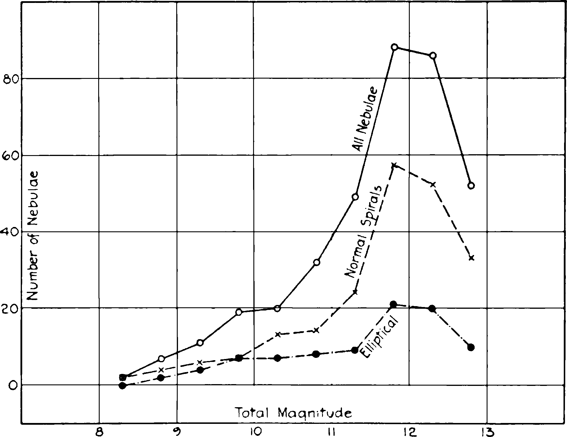
Fig. 1.—Frequency distribution of apparent magnitudes among nebulae in Holetschek’s list.
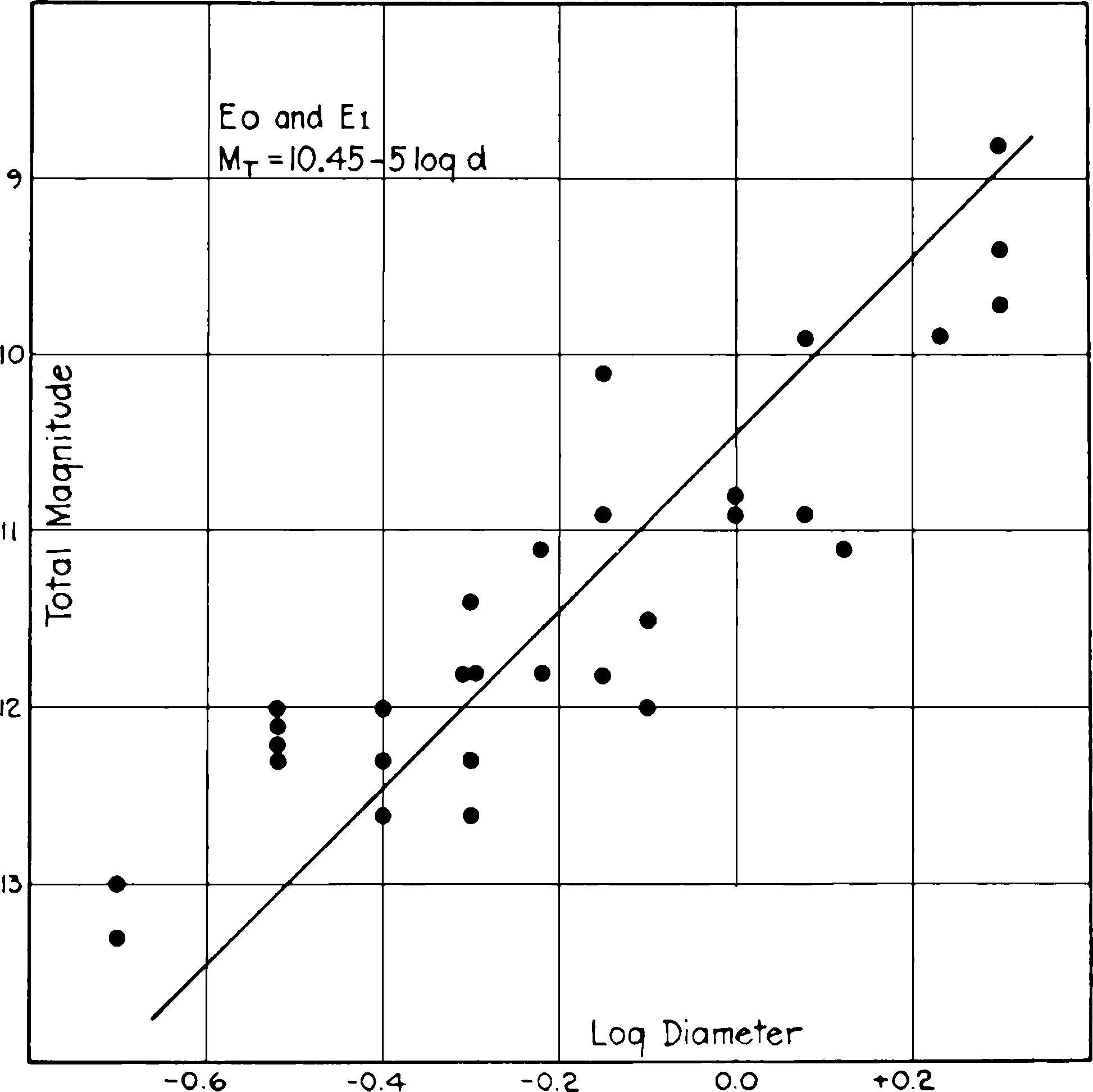
Fig. 2.—Relation between luminosity and diameter among nebulae at the beginning of the sequence of types—E0 and E1 nebulae.
The plot is shown in Figure 7, in which the two Magellanic{21} Clouds have been included in order to strengthen the bright end of the curve which would otherwise be unduly influenced by the single{22} object, M 31. The magnitudes +0.5 and +1.5, which were assigned to the Clouds, are estimates based upon published descriptions.
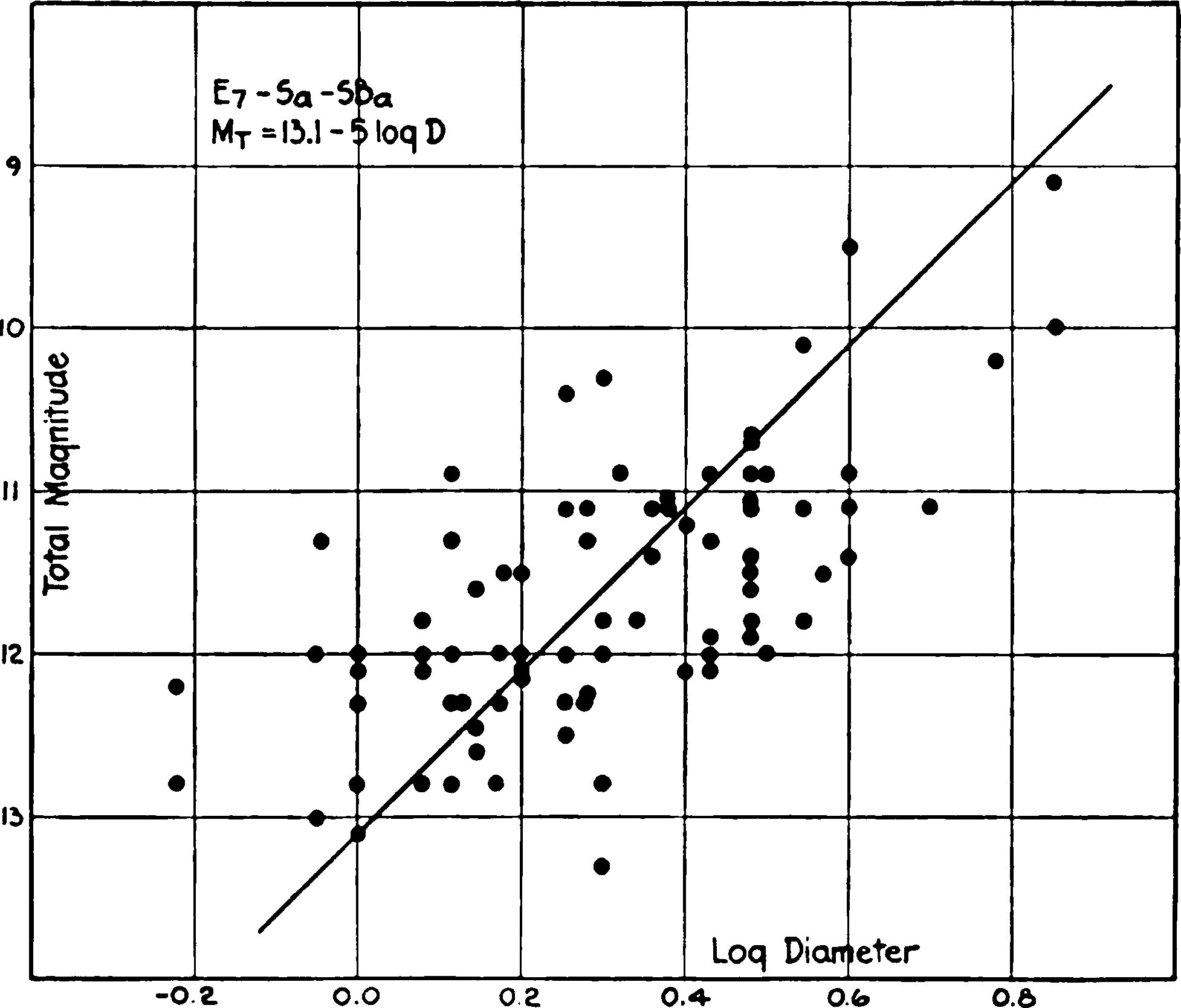
Fig. 3.—Relation between luminosity and diameter among nebulae at the middle of the sequence of types—E7, Sa, and SBa nebulae.
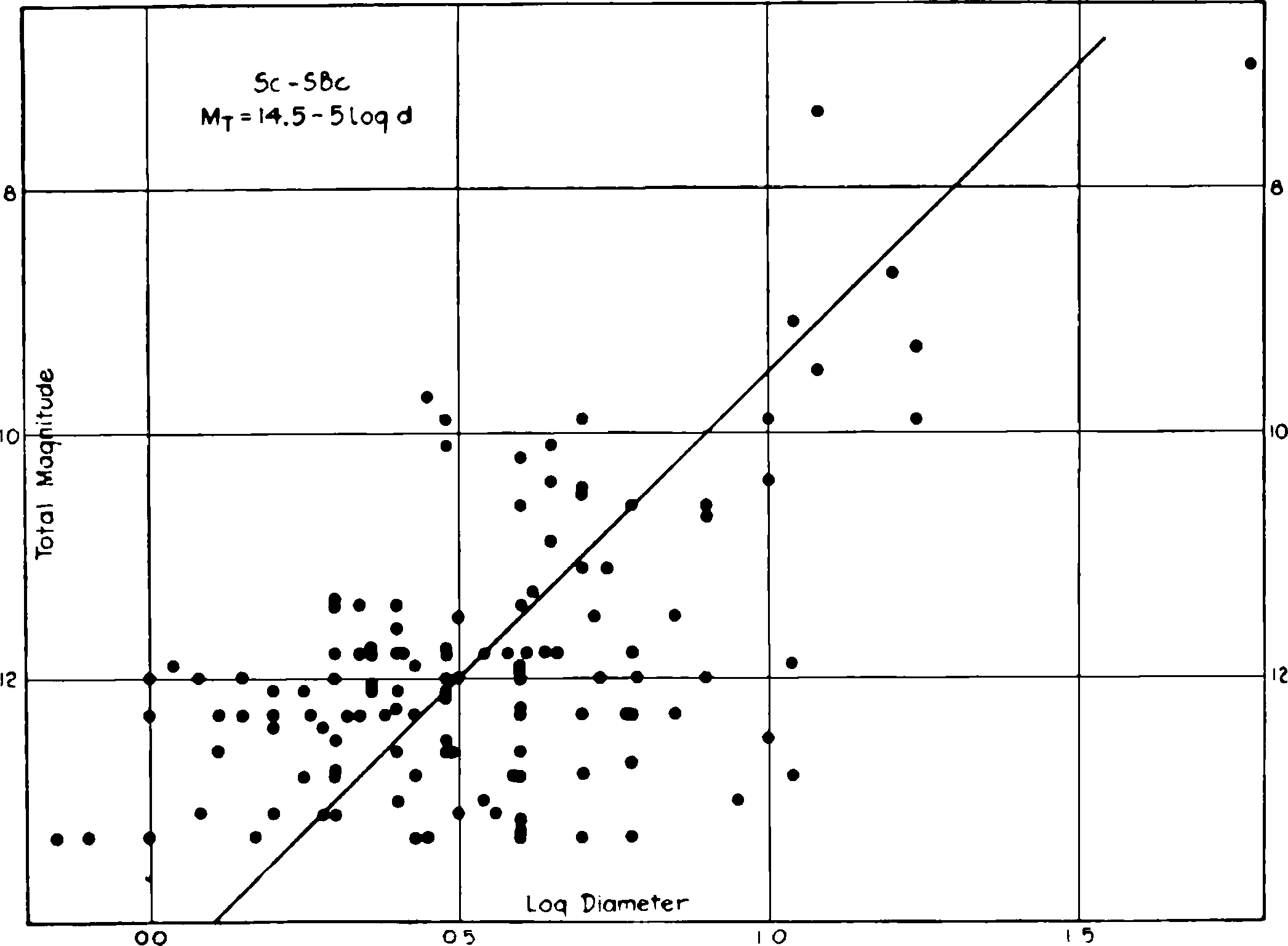
Fig. 4.—Relation between luminosity and diameter among nebulae at the end of the sequence of types—Sc and SBc nebulae.
The correlation of the data is very closely represented by the formula
 |
(2) |
This falls between the two regression curves derived from least-square solutions and could be obtained exactly by assigning appropriate weights to the two methods of grouping. The nature of the data is such that a closer agreement can scarcely be expected. No correction to the assumed value of the slope appears to be required. The material extends over a range of 12 mag., and the few cases which have been investigated indicate that the correlation can be extended another 3 mag., to the limit at which nebulae can be classified with certainty on photographs made with the 100-inch reflector. The relation may therefore be considered to hold throughout the entire range of observations.
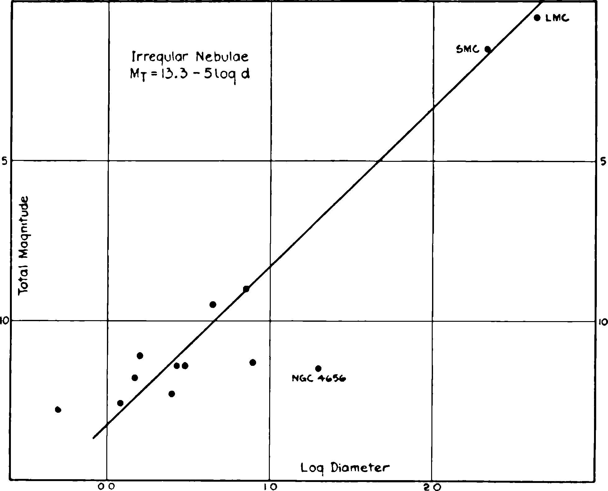
Fig. 5.—Relation between luminosity and diameter among the irregular nebulae. The Magellanic Clouds are included. N.G.C. 4656 is an exceptional case in that it shows a narrow, greatly elongated image in which absorption effects are very conspicuous; hence the maximum diameter is exceptionally large for its apparent luminosity.
{23}
The residuals without regard to sign average 0.87 mag., and there appears to be no systematic effect due either to type or luminosity. The scatter, however, is much greater for the spirals, especially in the later types, than for the elliptical nebulae. The limiting cases are explained by peculiar structural features. The nebulae which fall well above the line usually have bright stellar nuclei, and those which fall lowest are spirals seen edge-on in which belts of absorption are conspicuous.
TABLE VII
| Type | mT | log d | C* | d† |
|---|---|---|---|---|
| E0 | 11.40 | –0.204 | 10.38 | 1.2 |
| 1 | 11.43 | .177 | 10.54 | 1.3 |
| 2 | 11.52 | .088 | 11.08 | 1.6 |
| 3 | 11.99 | .133 | 11.33 | 1.8 |
| 4 | 11.95 | – .011 | 11.90 | 2.4 |
| 5 | 10.97 | + .090 | 11.42 | 1.9 |
| 6 | 10.93 | .220 | 12.03 | 2.5 |
| 7 | 11.02 | .360 | 12.82 | 3.7 |
| Sa | 11.69 | .333 | 13.35 | 4.7 |
| b | 11.55 | .471 | 13.90 | 6.0 |
| c | 11.74 | .540 | 14.44 | 7.7 |
| SBa | 11.66 | .267 | 13.00 | 4.0 |
| b | 11.48 | .317 | 13.16 | 4.3 |
| c | 11.87 | .509 | 14.41 | 7.6 |
| Irr | 11.34 | +0.469 | 13.68 | 5.4 |
* C = mT + 5 log d.
† log d = 0.2 (C — mT); mT = 10.0.
EFFECTS OF ORIENTATION
The effect of the orientation is appreciable among the spirals in general. In order to illustrate this feature, they have been divided into three groups consisting of those whose images are round or nearly round, elliptical, and edge-on, or nearly so. The mean values of mT + 5 log d were then computed and compared with the theoretical value, 13.0. The residuals are negative when the nebulae are too bright for their diameters and positive when they are too faint. The results are given in Table IX, where mean residuals are followed by the numbers of nebulae, in parentheses, which are represented by the means.
{24}
The numbers of the barred spirals are too limited to inspire confidence in the results, but among the normal spirals there is conclusive evidence that the highly tilted and edge-on nebulae are fainter for a given diameter than those seen in the round. A study of the individual images indicates that the effect is due very largely to dark absorption clouds, which become more conspicuous when the nebulae are highly tilted. These clouds are generally, but not universally, peripheral features. An extensive investigation will be necessary before any residual effect due to absorption by luminous nebulosity can be established with certainty. Even should such exist, it clearly cannot be excessive.
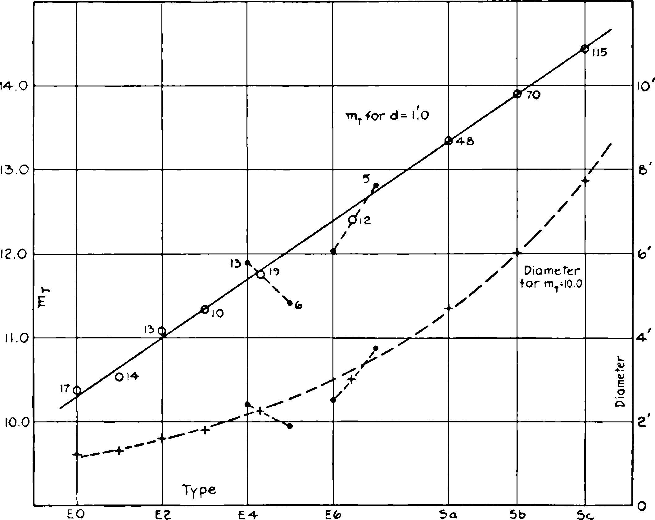
Fig. 6.—Progressive characteristics in the sequence of types. The upper curve represents the progression in total magnitude with type for nebulae having maximum diameters of one minute of arc. The elliptical nebulae and the normal spirals are included as representing the normal sequence, but the barred spirals and the irregular nebulae are omitted. The figures give the number of objects observed in each type. Among the later elliptical nebulae the numbers are so small that means of adjacent types have been plotted. The lower curve represents the progression in diameter along the normal sequence for nebulae of the tenth magnitude.
TABLE VIII
| Type | C | Δ log d |
|---|---|---|
| E0 | 10.30 | +0.54 |
| 1 | 10.65 | .47 |
| 2 | 11.00 | .40 |
| 3 | 11.35 | .33 |
| 4 | 11.70 | .26 |
| 5 | 12.05 | .19 |
| 6 | 12.40 | .12 |
| 7 | 12.75 | +0.05 |
| Sa | 13.31 | –0.06 |
| Sb | 13.90 | .18 |
| Sc | 14.45 | .29 |
| SBa | 13.00 | .00 |
| SBb | 13.16 | .03 |
| SBc | 14.41 | .28 |
| Irr | 13.68 | –0.14 |
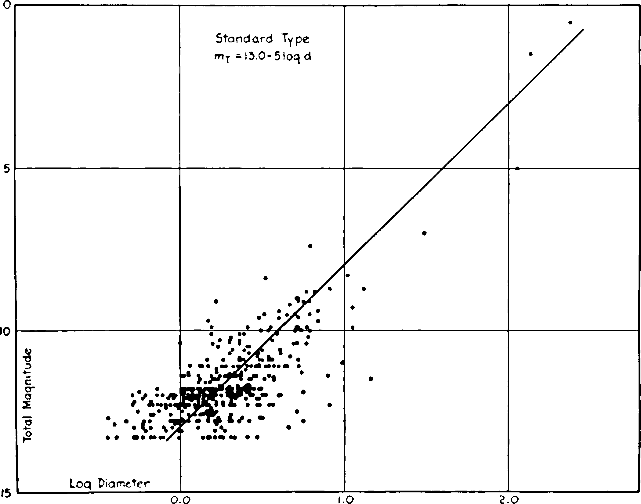
Fig. 7.—Relation between luminosity and diameter among extra-galactic nebulae. The nebulae have been reduced to a standard type, S0, which, being the mean of E7, Sa, and SBa, represents a hypothetical transition point between elliptical nebulae and spirals. The Magellanic Clouds have been included in order to strengthen the brighter end of the plot.
SIGNIFICANCE OF THE LUMINOSITY RELATION
The correlations thus far derived are between total luminosities and maximum diameters. In the most general sense, therefore, they{25} express laws of mean surface brightness. The value, K = 5.0, in formula (1) indicates that the surface brightness is constant for each separate type. The variations in C indicate a progressive diminution in the surface brightness from class to class throughout the entire sequence. The consistency of the results amply justifies the sequence as a basis of classification, since a progression in physical dimensions{26} is indicated, which accompanies the progression in structural form. Although the correlations do not necessarily establish any generic relation among the observed classes, they support in a very evident manner the hypothesis that the various stages in the sequence represent different phases of a single fundamental type of astronomical body. Moreover, the quantitative variation in C is consistent with this interpretation, as is apparent from the following considerations.
TABLE IX
Residuals in mT + 5 log d as a Function of Orientation
| Type | Round | Elliptical | Edge-On | |
|---|---|---|---|---|
| Sa | –0.02 (13) | –0.27 (13) | +0.57 (23) | |
| Sb | .77 (24) | .0 (35) | 1.71 (11) | |
| Sc | –0.08 (35) | –0.13 (57) | +0.66 (22) | |
| All S | –0.26 (72) | –0.11 (105) | +0.83 (56) | |
| SBa | 0.0 (10) | –0.30 (7) | +0.31 (8) | |
| SBb | – .16 (10) | + .07 (6) | ||
| SBc | +0.19 (9) | –0.50 (4) | +0.32 (2) | |
| All SB | +0.01 (29) | +0.21 (17) | +0.31 (10) | |
| All spirals | –0.22 (101) | –0.13 (122) | +0.73 (66) | |
Among the elliptical nebulae it is observed that the nuclei are sharp and distinct and that the color distribution is uniform over the images. This indicates that there is no appreciable absorption, either general or selective, and hence that the luminosity of the projected image represents the total luminosity of the nebula, regardless of the orientation. If the observed classes were pure, that is, if the apparent ellipticities were the actual ellipticities, formula (1) could be written
 |
(3) |
where b is the minor diameter in minutes of arc and e is the ellipticity. The term mT + 5 log b is observed to be constant for a given type. If it were constant for all elliptical nebulae, then the term Ce + 5 log (1 – e) would be constant also. On this assumption,
 |
{27} where C0 is the value of C for the pure class E0. Hence
 |
(4) |
a relation which can be tested by the observations. An analysis of the material indicates that this is actually the case, and hence that among the elliptical nebulae in general, the minor diameter determines the total luminosity, at least to a first approximation.18
The observed values of C vary with the class, as is seen in Table VII and Figure 6, but, excepting that for E7, they are too large because of the mixture of later types of nebulae among those of a given observed class. It is possible, however, to calculate the values of Ce – C0 for the pure classes and then to make approximate corrections for the observed mixtures on the assumption that the nebulae of any given actual ellipticity are oriented at random. In this manner, mean theoretical values can be compared with the observed values. The comparisons are shown in Table XII in the form C7 – Ce, because E7 is the only observed class that can be considered as pure. The significance of the table will be discussed later.
The following method has been used to determine the relative frequencies with which nebulae of a given actual ellipticity, oriented at random, will be observed as having various apparent ellipticities.
In Figure 8, let the co-ordinate axes OX and OY coincide with the major and minor axes, a and b, of a meridian section of an ellipsoid of revolution. Let OO′ be the line of sight to the observer, making an angle i with OX, and let OR be perpendicular to OO′. Let PP′ be a{28} tangent to the ellipse, parallel to and at a distance from OO′. Let x0 and y0 be the intercepts of the tangent on the X- and Y-axis, respectively. The apparent ellipticity is determined by bx, which, for various values of the angle i, ranges from b to a. The problem is to determine the relative areas on the surface of a sphere whose center is O, within which the radius OY must pass in order that the values of b1, and hence of the apparent ellipticity, e1 may fall within certain designated limits. This requires that the angle i be expressed in terms of b1.
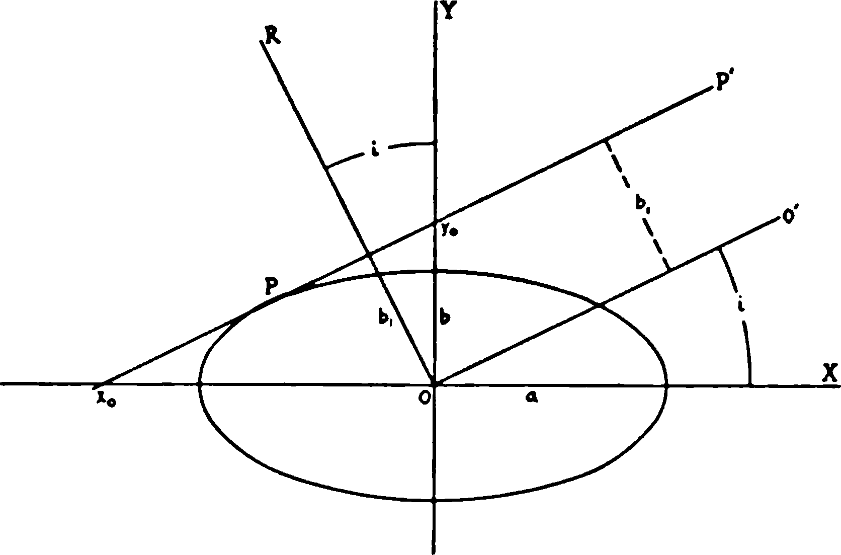
Fig. 8
From the equation of the tangent, PP′, 
 Since
Since 
 Let a = 1, then
  where
where 
From these equations, the values of i can be determined for all possible values of e1. The limits for the observed classes E0 to E7 were chosen midway between the consecutive tenths, E0 ranging{29} from e = 0 to e = 0.05; E1, from e = 0.05 to e = 0.15; E7, from e = 0.65 to e = 0.75. The relative frequencies of the various observed classes are then proportional to the differences in sin i corresponding to the two limiting values of e1. These frequencies must be calculated separately for nebulae of different actual ellipticities.
The results are given in Table X, where the actual ellipticities, listed in the first column, are followed across the table by the percentages which, on the assumption of random orientation, will be observed as having the various apparent ellipticities. The bottom row will be seen to show the percentages of apparent ellipticities observed in an assembly of nebulae in which the numbers for each actual ellipticity are equal and all are oriented at random.
TABLE X
| Actual | Apparent | ||||||||
|---|---|---|---|---|---|---|---|---|---|
| E0 | E1 | E2 | E3 | E4 | E5 | E6 | E7 | Total | |
| E7 | 0.055 | 0.111 | 0.114 | 0.116 | 0.121 | 0.132 | 0.164 | 0.187 | 1.000 |
| 6 | .059 | .123 | .126 | .133 | .148 | .187 | 0.224 | ||
| 5 | .067 | .140 | .148 | .166 | .216 | 0.263 | |||
| 4 | .079 | .169 | .190 | .250 | 0.312 | ||||
| 3 | .100 | .225 | .299 | 0.376 | |||||
| 2 | .145 | .378 | 0.477 | ||||||
| 1 | 0.300 | 0.700 | |||||||
| 0 | 1.000 | ||||||||
| Total | 1.805 | 1.846 | 1.354 | 1.041 | 0.797 | 0.582 | 0.388 | 0.187 | 8.000 |
| 0.226 | 0.231 | 0.169 | 0.130 | 0.100 | 0.073 | 0.049 | 0.023 | 1.000 | |
From this table and the actual numbers in the observed classes as read from a smoothed curve, the numbers of each actual ellipticity mingled in the observed classes can be determined. For instance, the four nebulae observed as E7 represent 0.187 of the total number of actual E7. The others are distributed among the observed classes E0 to E6 according to the percentages listed in Table X. Six nebulae are observed as E6, but 3.6 of these are actually E7. The remaining 2.4 actual E6 nebulae represent 0.224 of the total number of that actual ellipticity, the others, as before, being scattered among the observed classes E0 to E5. Table XI gives the complete analysis and is similar to Table X except that the percentages in the latter are replaced by the actual numbers indicated by the observations.
{30}
Finally, the mean values of C7 – Ce are calculated from the numbers of nebulae in the various columns of Table XI together with the values of C7 – Ce for the pure classes as derived from formula (4). The results are listed in the fourth column of Table XII following those for the pure and the observed classes. In determining the observed values, N.G.C. 524 and 3998 are included as E0 and E1, although in Table I they are listed as peculiar, because they are obviously much flattened nebulae whose minor axes are close to the line of sight.
TABLE XI
| Actual | Apparent | ||||||||
|---|---|---|---|---|---|---|---|---|---|
| E0 | E1 | E2 | E3 | E4 | E5 | E6 | E7 | Total | |
| E7 | 1.2 | 2.4 | 2.5 | 2.5 | 2.6 | 2.9 | 3.6 | 4.0 | 21.7 |
| 6 | 0.6 | 1.3 | 1.4 | 1.5 | 1.6 | 2.0 | 2.4 | 10.8 | |
| 5 | .8 | 1.7 | 1.8 | 2.0 | 2.7 | 3.1 | 12.1 | ||
| 4 | .8 | 1.7 | 1.9 | 2.5 | 3.1 | 10.0 | |||
| 3 | .9 | 2.1 | 2.8 | 3.5 | 9.3 | ||||
| 2 | 1.1 | 2.9 | 3.6 | 7.6 | |||||
| 1 | 1.7 | 3.9 | 5.6 | ||||||
| 0 | 9.9 | 9.9 | |||||||
| Total* | 17.0 | 16.0 | 14.0 | 12.0 | 10.0 | 8.0 | 6.0 | 4.0 | 87.0 |
* The totals represent the numbers in the observed classes as read from a smooth curve.
The observed values in general fall between those for the pure classes and those corresponding to random orientation. They are of the same order as the latter, and the discrepancies are perhaps not unaccountably large in view of the nature and the limited extent of the material. There is a systematic difference, however, averaging about 0.2 mag., in the sense that the observed values are too large, and increasing with decreasing ellipticity. One explanation is that the observed classes are purer than is expected on the assumption of random orientation. This view is supported by the relatively small dispersion in C, as may be seen in Table I and Figure 2, among the nebulae of a given class, but it is difficult to account for any such selective effect in the observations. The discrepancies may be largely eliminated by an arbitrary adjustment of the numbers of nebulae with various degrees of actual ellipticity; for instance, the values in{31} the last column of Table XII, calculated on the assumption of equal numbers, agree very well with the observed values, although the resulting numbers having the various apparent ellipticities differ slightly from those observed. The observed values, however, can again be accounted for by the inclusion of some flatter nebulae among the classes E6 and E7. Very early Sa or SBa nebulae might easily be mistaken for E nebulae when oriented edge-on, although they would be readily recognized when even slightly tilted. If the numerical results fully represented actual statistical laws, the explanation would be sought in the physical nature of the nebulae. The change from ellipsoidal to lenticular figures, noticeable in the later-type nebulae, would affect the results in the proper direction, as would also a progressive shortening of the polar axis. The discrepancies, however, are second-order effects, and since they may be due to accidental variations from random orientation, a further discussion must await the accumulation of more data.
TABLE XII
Differential Values of C
| Class | Pure Classes | Observed | Random Orientation | |
|---|---|---|---|---|
| No. as Observed | Equal No. | |||
| C7–C7 | 0.00 | 0.00 | 0.00 | 0.00 |
| C6 | 0.63 | 0.35* | 0.25 | 0.35 |
| C5 | 1.10 | 0.70* | 0.58 | 0.70 |
| C4 | 1.51 | 0.85 | 1.11 | 1.01 |
| C3 | 1.84 | 1.42 | 0.87 | 1.28 |
| C2 | 2.13 | 1.67 | 1.33 | 1.55 |
| C1 | 2.39 | 2.01† | 1.54 | 1.83 |
| C0 | 2.62 | 2.17† | 2.15 | 2.25 |
* Read from smooth curve in Fig. 6. The small numbers of observed E5 and E6 nebulae justify this procedure. The other values are the means actually observed.
† N.G.C. 524 and 3998 are included as E0 and E1, respectively.
Meanwhile, it is evident that, to a first approximation at least, the polar diameters alone determine the total luminosities of all elliptical nebulae, and the entire series can be represented by the various configurations of an originally globular mass expanding equatorially. A single formula represents the relation, in which the value of C is that corresponding to the pure type E0. From Table XII,{32} this is found to be 2.62 mag. less than the value of C7 The latter is observed to be 12.75, hence
 |
(5) |
If this relation held for the spirals as well, the polar diameters could be calculated from the measured magnitudes. Unfortunately, it has not been possible to measure accurately the polar diameters directly, and hence to test the question, but they have been computed for the mean magnitudes of the Sa, Sb, and Sc nebulae as given in Table III, and the ratios of the axes have been derived by a comparison of these hypothetical values with the means of the measured maximum diameters. The results, 1 to 4.4, 1 to 5.7, and 1 to 7.3, respectively, although of the right order, appear to be somewhat too high. An examination of the photographs indicates values of the order of 1 to 5.5, 1 to 8, and 1 to 10, but the material is meager and may not be representative. The comparison emphasizes, however, the homogeneity and the progressive nature of the entire sequence of nebulae and lends some additional color to the assumption that it represents various aspects of the same fundamental type of system.
From the dynamical point of view, the empirical results are consistent with the general order of events in Jeans’s theory. Thus interpreted, the series is one of expansion, and the scale of types becomes the time scale in the evolutionary history of nebulae. In two respects this scale is not entirely arbitrary. Among the elliptical nebulae the successive types differ by equal increments in the ellipticity or the degree of flattening, and among the spirals the intermediate stage is midway between the two end-stages in the structural features as well as in the luminosity relations.
One other feature of the curves may be discussed from the point of view of Jeans’s theory before returning to the strictly empirical attitude. The close agreement of the diameters for the stages E7 and Sa suggests that the transition from the lenticular nebula to the normal spiral form is not cataclysmic. If the transition were gradual, however, we should expect to observe occasional objects in the very process, but among the thousand or so nebulae whose images have been inspected, not one clear case of a transition form has been detected. The observations jump suddenly from lenticular nebulae{33} with no trace of structure to spirals in which the arms are fully developed.
If the numerical data could be fully trusted, the SBa forms would fill the gap. Among these nebulae, the transition from the lenticular to the spiral with arms is gradual and complete. It is tempting to suppose that the barred spirals do not form an independent series parallel with that of the normal spirals, but that all or most spirals begin life with the bar, although only a few maintain it conspicuously throughout their history. This would also account for the fact that the relative numbers of the SBa nebulae are intermediate to those of the lenticular and of the Sa. The normal spirals become more numerous as the sequence progresses, while the numbers of barred spirals, on the contrary, actually decrease with advancing type.
RELATION BETWEEN NUCLEAR LUMINOSITIES AND DIAMETERS
Visual magnitudes have been determined by Hopmann for the nuclei of 37 of the nebulae included in the present discussion. These data, together with types and diameters of the nebulae, are listed in Table XIII. When the magnitudes are plotted directly against the logarithms of the diameters, they show little or no correlation. When, however, the nebulae are reduced to the standard type (by applying corrections for differences in diameter along the sequence), a decided correlation is found whose coefficient is 0.76. This is shown in Figure 9 The simple mean of the two regression curves is
 |
(6) |
where the slope differs by about 1 per cent from that in formula (2). The list contains 16 elliptical nebulae, 15 normal, and 6 barred spirals. The nebulae are fairly representative, except that few late-type spirals are included. This is an effect of selection due to the fact that nuclei become less and less conspicuous as the sequence progresses.
The same result can be derived from a study of the differences, mn – mT, for the individual nebulae. The mean value is 1.55 ± 0.08, and the average residual is 0.60 mag. Means for the separate types are to be found in Table XIV.
TABLE XIII
Diameters and Nuclear Magnitudes
| N.G.C. | Type | log d | mn Hopmann | mn Reduced |
|---|---|---|---|---|
| 221 | E2 | +0.42 | 9.84 | 11.85 |
| 1023 | SBa | .78 | 11.86 | 11.86 |
| 2841 | Sb | 0.78 | 12.08 | 11.19 |
| 3031 | Sb | 1.20 | 10.94 | 10.05 |
| 3115 | E7 | 0.60 | 10.83 | 11.09 |
| 3351 | SBb | .48 | 12.31 | 12.15 |
| 3368 | Sa | .85 | 11.68 | 11.43 |
| 3379 | E0 | .30 | 11.55 | 14.27 |
| 3412 | SBa | .40 | 11.59 | 11.59 |
| 3489 | Sb | .40 | 11.54 | 10.65 |
| 3626 | Sa | .28 | 12.37 | 12.12 |
| 3627 | Sb | .90 | 12.03 | 11.14 |
| 4125 | E4 | .30 | 11.74 | 13.04 |
| 4216 | Sb | .85 | 11.65 | 10.76 |
| 4278 | E1 | .0 | 12.02 | 14.38 |
| 4374 | E1 | .08 | 11.43 | 13.79 |
| 4382 | E4 | .48 | 11.77 | 13.07 |
| 4435 | E6 | .11 | 11.65 | 12.26 |
| 4438 | Sb | .54 | 11.83 | 10.94 |
| 4486 | E0 | .30 | 11.23 | 13.95 |
| 4546 | E6 | .18 | 11.75 | 12.36 |
| 4552 | E0 | .23 | 11.59 | 14.31 |
| 4569 | Sc | .65 | 12.05 | 10.57 |
| 4579 | SBc | .45 | 11.48 | 10.07 |
| 4621 | E5 | .30 | 11.60 | 12.56 |
| 4636 | E1 | .08 | 11.97 | 14.33 |
| 4649 | E2 | .30 | 11.57 | 13.58 |
| 4697 | E6 | .48 | 10.90 | 11.51 |
| 4699 | SBb | .57 | 10.72 | 10.56 |
| 4725 | SBb | .70 | 11.97 | 11.81 |
| 4736 | Sb | .70 | 10.36 | 9.47 |
| 5005 | Sc | .70 | 12.04 | 10.56 |
| 5033 | Sc | 0.78 | 12.38 | 10.90 |
| 5194 | Sc | 1.08 | 11.38 | 9.90 |
| 5322 | E3 | 0.15 | 12.10 | 13.76 |
| 5866 | Sa | .48 | 11.76 | 11.51 |
| 7331 | Sb | +0.95 | 11.82 | 10.93 |
| Means | +0.509 | 11.60 | 11.90 |
The low value for Sa-SBa is due to N.G.C. 5866, for which the{34} magnitude difference of 0.06 is certainly in error, and the high value for Sc and SBc, to M 51, for which the difference of 3.98 mag. is not representative. The latter is accounted for in part by the fact that the mT refers to the combined magnitude of the main spiral and the outlying mass, N.G.C. 5195. When these two cases are discarded, the final mean becomes 1.52 ± 0.05, and the average residual, 0.52 mag., is consistent with the probable errors of the magnitude determinations.{35} The small numbers of objects within each class are insufficient for reliable conclusions concerning slight variations along the sequence. From the constancy of mn – mT, the relation expressed by formula (6) necessarily follows, the small difference in the constant being accounted for by the different methods of handling the data.
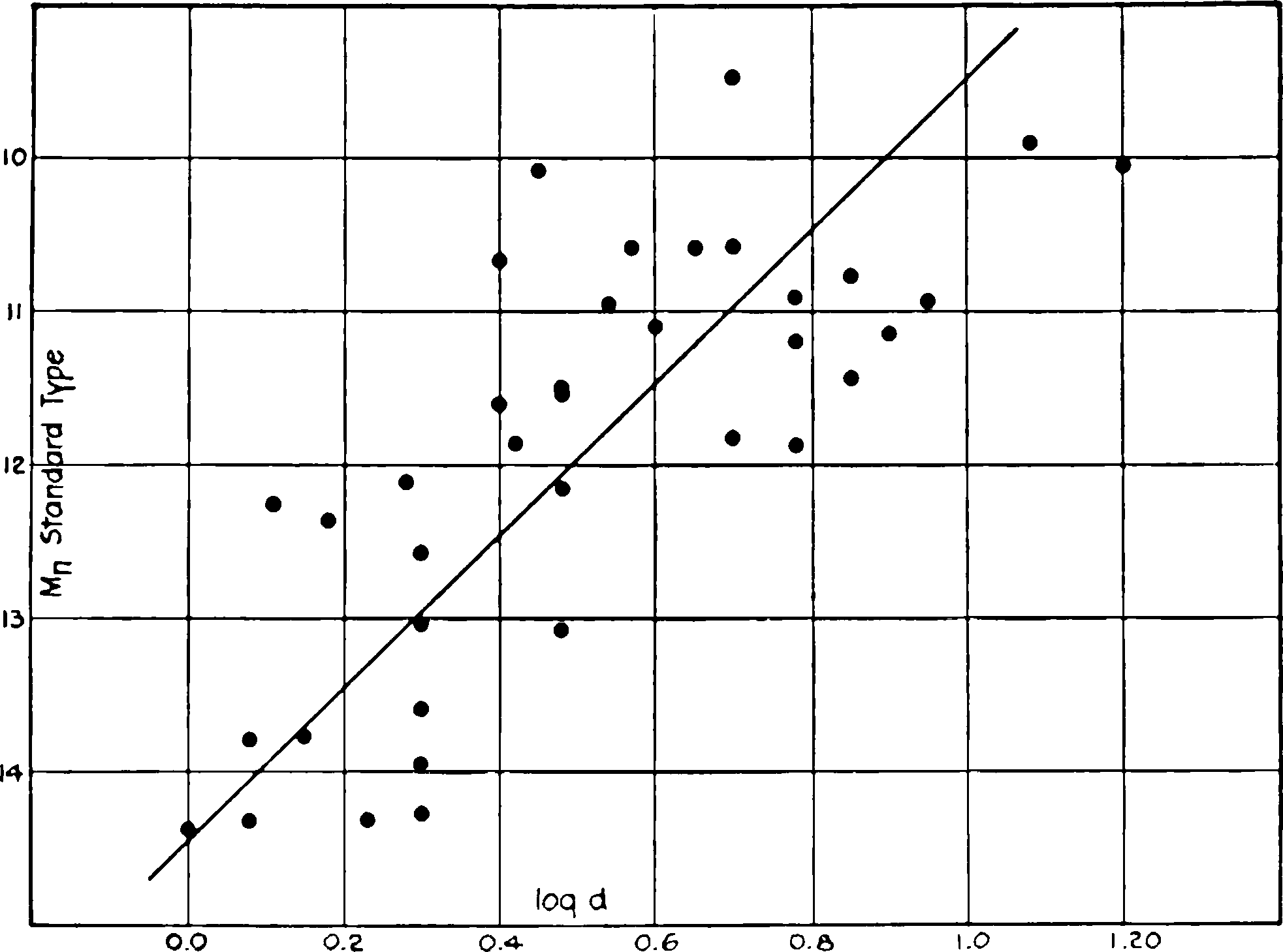
Fig. 9.—Relation between nuclear magnitudes and diameters. The nebulae have been reduced to the standard type by applying corrections to the magnitudes.
The parallelism of the two curves representing formulae (2) and (6) indicates that the regular extra-galactic nebulae, when reduced to the standard type, are similar objects. The mean surface brightness is constant, and the luminosity of the nucleus, as measured by Hopmann, is a constant fraction, about one-fourth, of the total luminosity of the nebulae. If there is a considerable range in absolute magnitude and hence in actual dimensions, the smaller nebulae must be faithful miniatures of the larger ones.
ABSOLUTE MAGNITUDES OF EXTRA-GALACTIC NEBULAE
Reliable values of distances, and hence of absolute magnitudes, are restricted to a very few of the brightest nebulae. These are derived from a study of individual stars involved in the nebulae, among which certain types have been identified whose absolute magnitudes in the galactic system are well known. The method assumes that the{36} stars involved in the nebulae are directly comparable with the stars in our own system, and this is supported by the consistency of the results derived from the several different types which have been identified.
TABLE XIV
| Type | mn – mT | Number | |
|---|---|---|---|
| E0–E3 | 1.64 | (9) | |
| E4–E7 | 1.43 | (7) | |
| Sa–SBa | 0.97 | (5) | 1.27 when N.G.C. 5866 is omitted |
| Sb–SBb | 1.70 | (11) | |
| Sc–SBc | 1.76 | (5) | 1.19 when N.G.C. 5194 is omitted |
| Unweighted mean | 1.50 | (37) | 1.45 (35) |
| Weighted mean | 1.55 | (37) | 1.52 (35) |
TABLE XV
Absolute Magnitudes of Nebulae
| System | MT | MS |
|---|---|---|
| Galaxy | –5.5 | |
| M 31 | –17.1 | 6.5 |
| LMC | 17.0 | 8.0 |
| SMC | 16.0 | 5.5 |
| M 33 | 15.1 | 6.5 |
| N.G.C. 6822 | 13.7 | 5.8 |
| M 101 | 13.5 | –6.3 |
| M 32 | –13.3 | |
| –6.3 | ||
| –9.0 = MS – MT | ||
| Means | –15.1 | –15.3 |
| Adopted | –15.2 |
In Table XV are listed absolute magnitudes of the entire system and of the brightest stars involved, for the galaxy and the seven nebulae whose distances are known. The data for the Magellanic Clouds are taken from Shapley’s investigations. The absolute magnitudes of the remaining nebulae were derived from Holetschek’s apparent magnitudes and the distances as determined at Mount Wilson, where the stellar magnitudes were also determined. M 32 is generally assumed to be associated with the great spiral M 31, because the radial velocities are nearly equal and are unique in that{37} they are the only large negative velocities that have been found among the extra-galactic nebulae. M 101 has been added to the list on rather weak evidence. The brightest stars involved are slightly brighter than apparent magnitude 17.0, and several variables have been found with magnitudes at maxima fainter than 19.0. Sufficient observations have not yet been accumulated to determine the light-curves of the variables, but from analogy with the other nebulae they are presumed to be Cepheids. On this assumption, both the star counts and the variables lead to a distance of the order of 1.7 times the distance of M 33. The inclusion of M 101 does not change the mean magnitude of the brightest stars involved, but reduces the mean magnitude of the nebulae by 0.2.
The range in the stars involved is about 2.5 mag., and in the total luminosities of the nebulae, about 3.8 mag. This latter is consistent with the scatter in the diagram exhibiting the relation between total luminosities and diameters. The associated objects, M 31 and 32, represent the extreme limits among the known systems, and the mean of these two is very close to the mean of them all.
LUMINOSITY OF STARS INVOLVED IN NEBULAE
The number of nebulae of known distance is too small to serve as a basis for estimates of the range in absolute magnitude among nebulae in general. Further information, however, can be derived from a comparison of total apparent magnitudes with apparent magnitudes of the brightest stars involved, on the reasonable assumption, supported by such evidence as is available, that the brightest stars in isolated systems are of about the same intrinsic luminosity.
The most convenient procedure is to test the constancy of the differences in apparent magnitude between the brightest stars involved and the nebulae themselves, over as wide a range as possible in the latter quantities.
An examination of the photographs in the Mount Wilson collection has revealed no stars in the very faint objects or in the bright elliptical nebulae and early-type spirals. This was to be expected from the conclusions previously derived. Observations were therefore confined to intermediate- and late-type spirals and the irregular{38} nebulae to the limiting visual magnitude 10.5. The Magellanic Clouds and N.G.C. 6822 were added to the nebulae in Holetschek’s{39} list. Altogether, data were available for 32 objects, or about 60 per cent of the total number in the sky to the adopted limit. For this reason it is believed that the results are thoroughly representative.
TABLE XVI
Difference in Magnitude between Nebulae and Their Brightest Stars
| N.G.C. | ms | mT | ms – mT |
|---|---|---|---|
| Sb | |||
| 224 | 15.5 | 5.0 | 10.5 |
| 1068 | 17.5 | 9.1 | 8.4 |
| 2841 | >19.5 | 9.4 | >10.1 |
| 3031 | 18.5 | 8.3 | 10.2 |
| 3310 | >19.0 | 10.4 | > 8.6 |
| 3623 | >20.0 | 9.9 | >10.1 |
| 3627 | 18.5 | 9.1 | 9.4 |
| 4438 | >19.0 | 10.3 | > 8.7 |
| 4450 | 19.5 | 10.0 | 9.5 |
| 4736 | 17.3 | 8.4 | 8.9 |
| 4826 | >19.5 | 9.2 | >10.3 |
| 5055 | >19.0 | 9.6 | > 9.4 |
| 5746 | >19.5 | 10.4 | > 9.1 |
| 7331 | 19.0 | 10.4 | 8.6 |
| SBb | |||
| 4699 | >19.5 | 10.0 | > 9.5 |
| Sc | |||
| 253 | 18.3 | 9.3 | 9.0 |
| 598 | 15.6 | 7.0 | 8.6 |
| 2403 | 17.3 | 8.7 | 8.6 |
| 2683 | >20.0 | 9.9 | >10.1 |
| 2903 | 19.0 | 9.1 | 9.9 |
| 4254 | 18.5 | 10.4 | 8.1 |
| 4321 | 18.8 | 10.5 | 8.3 |
| 4414 | >19.5 | 10.1 | > 9.4 |
| 4490 | 18.8 | 10.2 | 8.6 |
| 5194 | 17.3 | 7.4 | 9.9 |
| 5236 | 18.6 | 10.4 | 8.2 |
| 5457 | 17.0 | 9.9 | 7.1 |
| Irr. | |||
| LMC | 9.5 | 0.5 | 9.0 |
| SMC | 12.0 | 1.5 | 10.5 |
| 3034 | >19.5 | 9.0 | >10.5 |
| 4449 | 17.8 | 9.5 | 8.3 |
| 6822 | 15.8 | 8.5 | 7.3 |
The data are listed in Table XVI and are shown graphically in Figure 10. The luminosities of the brightest stars are given in photographic magnitudes. For the Magellanic Clouds, M 33, and N.G.C. 6822, these were obtained from published star counts. For M 31, 51, 63, 81, 94, and N.G.C. 2403, they depend upon unpublished counts, for which the magnitudes were determined by comparisons with Selected Areas. For the remaining nebulae, the magnitudes of stars were estimated with varying degrees of precision, but are probably less than 0.5 mag. in error.
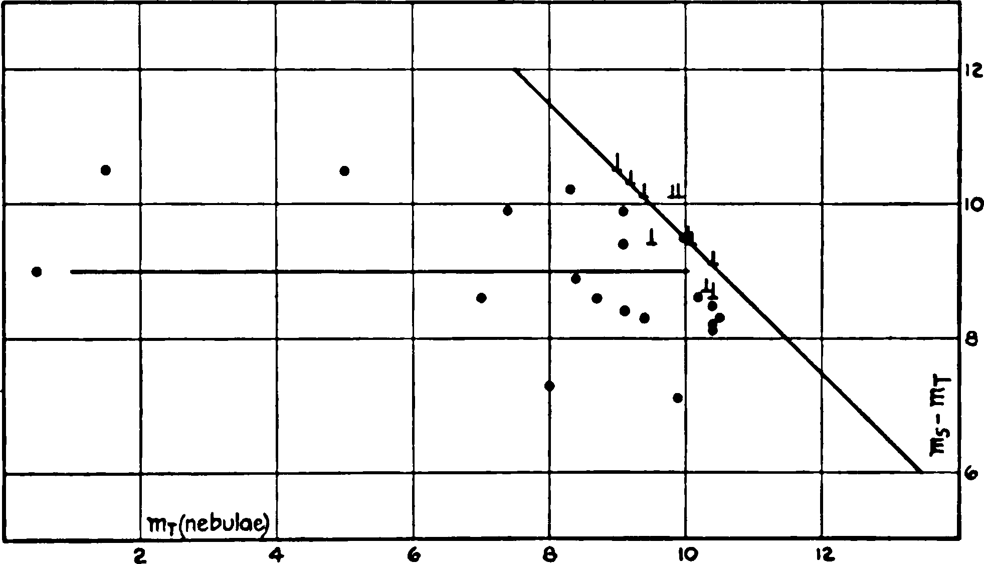
Fig. 10.—Relation between total magnitudes of extra-galactic nebulae and magnitudes of the brightest stars involved. Differences between total visual magnitudes of nebulae and the photographic magnitudes of the brightest stars are plotted against the total magnitudes. The dots represent cases in which the stars could actually be detected; the incomplete crosses represent cases in which stars could not be detected, and hence give lower limits for the magnitude differences. The diagonal line indicates the approximate limits of observation, fixed by the circumstance that, in general, stars fainter than 19.5 probably would not be detected on the nebulous background.
The sloping line to the right in Figure 10 represents the limits of the observations, for, from a study of the plates themselves, it appeared improbable that stars fainter than about 19.5 could be detected with certainty on a nebulous background. Points representing nebulae in which individual stars could not be found should lie in this excluded region above the line, and their scatter is presumably{40} comparable with that of the points actually determined below the line. When allowance is made for this inaccessible region, the data can be interpreted as showing a moderate dispersion around the mean ordinate
 |
(7) |
The range in total magnitudes is sufficiently large in comparison with the dispersion to lend considerable confidence to the conclusion. The total range of four, and the average dispersion of less than 1 mag., are comparable with those in Table XV and in Figure 7, and agree with the former in indicating a constant order of absolute magnitude.
The mean absolute magnitude of the brightest stars in the nebulae listed in Table XV, combined with the mean difference between nebulae and their brightest stars, furnishes a mean absolute magnitude of –15.3 for the nebulae listed in Table XVI. This differs by only 0.2 mag. from the average of the nebulae in Table XV, and the mean of the two, –15.2, can be used as the absolute magnitude of intermediate- and late-type spirals and irregular nebulae whose apparent magnitudes are brighter than 10.5. The dispersion is small and can safely be neglected in statistical investigations.
This is as far as the positive evidence can be followed. For reasons already given, however, it is presumed that the earlier nebulae, the elliptical and the early-type spirals, are of the same order of absolute magnitude as the later. The one elliptical nebula whose distance is known, M 32, is consistent with this hypothesis.
Conclusions concerning the intrinsic luminosities of the apparently fainter nebulae are in the nature of extrapolations of the results found for the brighter objects. When the nebulae are reduced to a standard type, they are found to be constructed on a single model, with the total luminosities varying directly as the square of the diameters. The most general interpretation of this relation is that the mean surface brightness is constant, but the small range in absolute magnitudes among the brighter nebulae indicates that, among these objects at least, the relation merely expresses the operation of the inverse-square law on comparable objects distributed at different distances. The actual observed range covered by this restricted interpretation is from apparent magnitude 0.5 to 10.5. The{41} homogeneity of the correlation diagrams and the complete absence of evidence to the contrary justify the extrapolation of the restricted interpretation to cover the 2 or 3 mag. beyond the limits of actual observation.
These considerations lead to the hypothesis that the nebulae treated in the present discussion are all of the same order of absolute magnitude; in fact, they lend considerable color to the assumption that extra-galactic nebulae in general are of the same order of absolute magnitude and, within each class, of the same order of actual dimensions. Some support to this assumption is found in the observed absence of individual stars in the apparently fainter late-type nebulae. If the luminosity of the brightest stars involved is independent of the total luminosity of a nebula, as is certainly the case among the brighter objects, then, when no stars brighter than 19.5 are found, the nebulae must in general be brighter than absolute magnitude mT – 25.8 where mT is the total apparent magnitude. On this assumption, the faintest of the Holetschek nebulae are brighter than –12.5 and hence of the same general order as the brighter nebulae.
Once the assumption of a uniform order of luminosity is accepted as a working hypothesis, the apparent magnitudes become, for statistical purposes, a measure of the distances. For a mean absolute magnitude of –15.2, the distance in parsecs is
 |
(8) |
DIMENSIONS OF EXTRA-GALACTIC NEBULAE
When the distances are known, it is possible to derive actual dimensions and hence to calibrate the curve in Figure 6, which exhibits the apparent diameters as a function of type, or stage in the nebular sequence, for nebulae of a given apparent magnitude. The mean maximum diameters in parsecs corresponding to the different mean types are given in Table XVII. For the elliptical nebulae, values are given both for the statistical mean observed diameters and for the diameter as calculated for the pure types.
Spirals at the last stage in the observed sequence have diameters of the order of 3000 parsecs. Assuming 1:10 as the ratio of the two{42} axes, the corresponding volume is of the order of 1.4×10⁹ cubic parsecs, and the mean luminosity density is of the order of 7.7 absolute magnitudes per cubic parsec as compared with 8.15 for the galactic system in the vicinity of the sun. These results agree with those of Seares who, from a study of surface brightness, concluded that the galactic system must be placed at the end of, if not actually outside, the series of known spirals when arranged according to density.19
TABLE XVII
| Type | Diameter in Parsecs | |
|---|---|---|
| Obs | Cal. | |
| E0 | 360 | 340 |
| E1 | 430 | 380 |
| E2 | 500 | 430 |
| E3 | 590 | 490 |
| E4 | 700 | 570 |
| E5 | 810 | 680 |
| E6 | 960 | 850 |
| E7 | 1130 | 1130 |
| Type | Diameter in Parsecs |
|---|---|
| Sa | 1450 |
| Sb | 1900 |
| Sc | 2500 |
| SBa | 1280 |
| SBb | 1320 |
| SBc | 2250 |
| Irr | 1500 |
MASSES OF EXTRA-GALACTIC NEBULAE
Spectroscopic rotations are available for the spirals M 3120 and N.G.C. 4594,21 and from these it is possible to estimate the masses on the assumption of orbital rotation around the nucleus. The distances of the nebulae are involved, however, and this is known accurately only for M 31; for N.G.C. 4594 it must be estimated from the apparent luminosity.
Another method of estimating masses is that used by Öpik22 in deriving his estimate of the distance of M 31. It is based on the assumption that luminous material in the spirals has about the same coefficient of emission as the material in the galactic system. Öpik computed the ratio of luminosity to mass for our own system in{43} terms of the sun as unity, using Jeans’s value23 for the relative proportion of luminous to non-luminous material. The relation is
| Mass = 2.6 L. | (9) |
The application of this method of determining orders of masses seems to be justified, at least in the case of the later-type spirals and irregular nebulae, by the many analogies with the galactic system itself. Moreover, when applied to M 31, where the distance is fairly well known, it leads to a mass of the same order as that derived from the spectrographic rotation:
MASS OF M 31
| Spectrographic rotation | 3.5×10⁹ ☉ |
| Öpik’s method | 1.6×10⁹ |
The distance of N.G.C. 4594 is unknown, but the assumption that it is a normal nebula with an absolute magnitude of –15.2 places it at 700,000 parsecs. The orders of the mass by the two methods are then
MASS OF N.G.C. 4594
| Spectrographic rotation | 2.0×10⁹ ☉ |
| Öpik’s method | 2.6×10⁸ |
Here again the resulting masses are of the same order. They can be made to agree as well as those for M 31 by the not unreasonable assumption that the absolute luminosity of the nebula is 2 mag. or so brighter than normal.
Öpik’s method leads to values that are reasonable and fairly consistent with those obtained by the independent spectrographic method. Therefore, in the absence of other resources, its use for deriving the mass of the normal nebula appears to be permissible. The result, 2.6 × 10⁸ ☉, corresponding to an absolute magnitude of –15.2, is probably of the right order. The two test cases suggest that this value may be slightly low, but the data are not sufficient to warrant any empirical corrections.
NUMBERS OF NEBULAE TO DIFFERENT LIMITING MAGNITUDES
The numbers of nebulae to different limiting magnitudes can be used to test the constancy of the density function, or, on the hypothesis{44} of uniform luminosities, to determine the distribution in space. The nebulae brighter than about the tenth magnitude are known individually. Those not included in Holetschek’s list are: the Magellanic Clouds, the two nebulae N.G.C. 55 and 1097, between 9.0 and 9.5 mag., and the seven nebulae N.G.C. 134, 289, 1365, 1533, 1559, 1792, and 3726, all between 9.5 and 10.0 mag.
A fair estimate of the number between 10.0 and 11.0 mag. can be derived from a comparison of Holetschek’s list with that of Hardcastle, an inspection of images on the Franklin-Adams charts and other photographs, and a correlation between known total magnitudes and the descriptions of size and brightness in Dreyer’s catalogues. It appears that very few of these objects were missed by Holetschek in the northern sky—not more than six of Hardcastle’s nebulae. For the southern sky, beyond the region observed by Holetschek, the results are very uncertain, but probable upper and lower limits were determined as 50 and 20, respectively. The brighter nebulae are known to be scarce in those regions. A mean value of 35 leads to a total 295 for the entire sky, and this is at least of the proper order.
The number of nebulae between 11.0 and 12.0 mag. can be estimated on the assumption that the two lists, Holetschek’s and Hardcastle’s, are about equally complete within this range. They are known to be comparable for the brighter nebulae, and, moreover, the total numbers included in the two lists for the same area of the sky, that north of declination –10°, are very nearly equal—400 as compared with 408. The percentages of Holetschek’s nebulae included by Hardcastle were first determined as a function of magnitude. Within the half-magnitude interval 11.0 to 11.5, for instance, 60 per cent are in Hardcastle’s list. If the two lists are equally complete and, taken together, are exhaustive, the total number in the interval will be 1.4 times the number of Holetschek’s nebulae. The latter is found to be 50 from smoothed frequency curves of the magnitudes listed in Tables I–IV. The total number north of –10° is therefore 70. This can be corrected to represent the entire sky by applying the factor 1.75, which is the ratio of the total number of Hardcastle’s nebulae, 700, to the number north of –10°, 400. In this manner a reasonable estimate of 123 is obtained for the number of nebulae in{45} the entire sky between 11.0 and 11.5 mag. Similarly, between 11.5 and 12.0, where 50 per cent of Holetschek’s nebulae are included in Hardcastle’s list, the total number for the entire sky is found to be 236.
The greatest uncertainty in these figures arises from the assumption that the two lists together are complete to the twelfth magnitude. The figures are probably too small, but no standards are available by which they can be corrected. It is believed, however, that the errors are certainly less than 50 per cent and probably not more than 25 per cent. This will not be excessive in view of the possible deviations from uniform distribution where so limited a number of objects is considered.
Beyond 12.0 mag. the lists quickly lose their aspect of completeness and cannot be used for the present purpose. There are available, however, the counts by Fath24 of nebulae found on plates of Selected Areas made with the 60-inch reflector at Mount Wilson. The exposures were uniformly 60 minutes on fast plates and cover the Areas in the northern sky down to and including the –15° zone. The limiting photographic magnitudes for stars average about 18.5. The counts have been carefully revised by Seares25 and are the basis for his estimate of 300,000 nebulae in the entire sky down to this limit.
Approximate limiting total magnitudes for the nebulae in two of the richest fields, S.A. 56 and 80, have been determined from extra-focal exposures with the 100-inch reflector. The results are 17.7 in each case, and this, corrected by the normal color-index of such objects, gives a limiting visual magnitude of about 16.7, which can be used for comparison with the counts of the brighter nebulae.
The various data are collected in Table XVIII, where the observed numbers of extra-galactic nebulae to different limits of visual magnitude are compared with those computed on the assumption of uniform distribution of objects having a constant absolute luminosity. The formula used for the computation is
 |
(10) |
{46} where the constant is the value of log N for mT = 0. The value —4.45 is found to fit the observational data fairly well.
The agreement between the observed and computed log N over a range of more than 8 mag. is consistent with the double assumption of uniform luminosity and uniform distribution or, more generally, indicates that the density function is independent of the distance.
The systematic decrease in the residuals O – C with decreasing luminosity is probably within the observational errors, but it may also be explained as due to a clustering of nebulae in the vicinity of the galactic system. The cluster in Virgo alone accounts for an appreciable part. This is a second-order effect in the distribution, however, and will be discussed at length in a later paper.
TABLE XVIII
Numbers of Nebulae to Various Limits
| mT | log N* | O – C | log D† | |
|---|---|---|---|---|
| O | C | |||
| 8.5 | 0.85 | 0.65 | +0.20 | 5.74 |
| 9.0 | 1.08 | 0.95 | .13 | 5.84 |
| 9.5 | 1.45 | 1.25 | .20 | 5.94 |
| 10.0 | 1.73 | 1.55 | .18 | 6.04 |
| 10.5 | 1.95 | 1.85 | .10 | 6.14 |
| 11.0 | 2.17 | 2.15 | + .02 | 6.24 |
| 11.5 | 2.43 | 2.45 | – .02 | 6.34 |
| 12.0 | 2.70 | 2.75 | .05 | 6.44 |
| 16.7 | 5.48 | 5.57 | –0.09 | 7.38 |
| (18.0) | (6.35) | (7.64) | ||
* Log N = 0.6 mT – 4.45.
† Log D = 0.2 mT + 4.04.
Distances corresponding to the different limiting magnitudes, as derived from formula (8), are given in the last column of Table XVIII. The 300,000 nebulae estimated to the limits represented by an hour’s exposure on fast plates with the 60-inch reflector appear to be the inhabitants of space out to a distance of the order of 2.4 × 10⁷ parsecs. The 100-inch reflector, with long exposures under good conditions, will probably reach the total visual magnitude 18.0, and this, by a slight extrapolation, is estimated to represent a distance of the order of 4.4×10⁷ parsecs or 1.4×10⁸ light-years, within which it is expected that about two million nebulae should be found. This{47} seems to represent the present boundaries of the observable region 3 of space.
DENSITY OF SPACE
The data are now available for deriving a value for the order of the density of space. This is accomplished by means of the formulae for the numbers of nebulae to a given limiting magnitude and for the distance in terms of the magnitude. In nebulae per cubic parsec, the density is
 |
(11) |
This is a lower limit, for the absence of nebulae in the plane of the Milky Way has been ignored. The current explanation of this phenomenon in terms of obscuration by dark clouds which encircle the Milky Way is supported by the extra-galactic nature of the nebulae, their general similarity to the galactic system, and the frequency with which peripheral belts of obscuring material are encountered among the spirals. The known clouds of dark nebulosity are interior features of our system, and they do not form a continuous belt. In the regions where they are least conspicuous, however, the extra-galactic nebulae approach nearest to the plane of the Milky Way, many being found within 10°. This is consistent with the hypothesis of a peripheral belt of absorption.
The only positive objection which has been urged to this explanation has been to the effect that the nebular density is a direct function of galactic latitude. Accumulating evidence26 has failed to confirm this view and indicates that it is largely due to the influence of the great cluster in Virgo, some 15° from the north galactic pole. There is no corresponding concentration in the neighborhood of the south pole.{48}
If an outer belt of absorption is assumed, which, combined with the known inner clouds, obscures extra-galactic nebulae to a mean distance of 15° from the galactic plane, the value derived for the density of space must be increased by nearly 40 per cent. This will not change the order of the value previously determined and is within the uncertainty of the masses as derived by Öpik’s method. The new value is then
| ρ = 9×10–18 nebulae per cubic parsec. | (12) |
The corresponding mean distance between nebulae is of the order of 570,000 parsecs, although in several of the clusters the distances between members appear to be a tenth of this amount or less.
The density can be reduced to absolute units by substituting the value for the mean mass of a nebula, 2.6×10⁸ ☉. Then, since the mass of the sun in grams is 2×1033 and 1 parsec is 3.1×1018 cm,
| ρ = 1.5×10⁻³¹ grams per cubic centimeter. | (13) |
This must be considered as a lower limit, for loose material scattered between the systems is entirely ignored. There are no means of estimating the order of the necessary correction. No positive evidence of absorption by inter-nebular material, either selective or general, has been found, nor should we expect to find it unless the amount of this material is many times that which is concentrated in the systems.
THE FINITE UNIVERSE OF GENERAL RELATIVITY
The mean density of space can be used to determine the dimensions of the finite but boundless universe of general relativity. De Sitter27 made the calculations some years ago, but used values for the density, 10–26 and greater, which are of an entirely different order from that indicated by the present investigations. As a consequence, the various dimensions, both for spherical and for elliptical space, were small as compared with the range of existing instruments.
For the present purpose, the simplified equations which Einstein has derived for a spherically curved space can be used.28 When{49} R, V, M, and ρ represent the radius of curvature, volume, mass, and density, and k and c are the gravitational constant and the velocity of light,
 |
(14) |
 |
(15) |
 |
(16) |
Substituting the value found for ρ, 1.5×10⁻³¹, the dimensions become
| R = 8.5×1028 cm = 2.7×10¹⁰ parsecs, | (17) |
| V = 1.1×1088 cm = 3.5×1032 cubic parsecs, | (18) |
| M = 1.8×1057 grams = 9×10²² ☉. | (19) |
The mass corresponds to 3.5×10¹⁵ normal nebulae.
The distance to which the 100-inch reflector should detect the normal nebula was found to be of the order of 4.4×1075 parsecs, or about 1⁄600 the radius of curvature. Unusually bright nebulae, such as M 31, could be photographed at several times this distance, and with reasonable increases in the speed of plates and size of telescopes it may become possible to observe an appreciable fraction of the Einstein universe.
Mount Wilson Observatory
September 1926
Meanwhile K. Lundmark, who was present at the Cambridge meeting and has since been appointed a member of the Commission, has recently published (Arkiv für Matematik, Astronomi och Fysik, Band 19B, No. 8, 1926) a classification, which, except for nomenclature, is practically identical with that submitted by me. Dr. Lundmark makes no acknowledgments or references to the discussions of the Commission other than those for the use of the term “galactic.”
An accepted precedent for this usage is found in the series of stellar spectral types. There also the progression is assumed to be from the simple to the complex, and in view of the great convenience of the terms “early” and “late,” the temporal connotations, after a full consideration of their possible consequences, have been deliberately disregarded.
| e | Ce | 5 log (1 – e) | C0 | Res. |
|---|---|---|---|---|
| 0 | 10.30 | 0.0 | 10.30 | –0.14 |
| 1 | 10.65 | – .23 | 10.42 | – .02 |
| 2 | 11.00 | .48 | 10.52 | + .10 |
| 3 | 11.35 | 0.78 | 10.57 | + .13 |
| 4 | 11.70 | 1.11 | 10.59 | + .15 |
| 5 | 12.05 | 1.50 | 10.55 | + .11 |
| 6 | 12.40 | 1.99 | 10.41 | – .03 |
| 7 | 12.75 | –2.62 | 10.13 | –0.31 |
| Mean | 10.44 | 0.12 |
Hellenica World - Scientific Library
Retrieved from "http://en.wikipedia.org/"
All text is available under the terms of the GNU Free Documentation License
