Nash equilibrium

In game theory, the Nash equilibrium, named after the mathematician John Forbes Nash Jr., is a proposed solution of a non-cooperative game involving two or more players in which each player is assumed to know the equilibrium strategies of the other players, and no player has anything to gain by changing only their own strategy.[1]

If each player has chosen a strategy—an action plan choosing its own action based on what it has seen happen so far in the game—and no player can increase its own expected payoff by changing its strategy while the other players keep theirs unchanged, then the current set of strategy choices constitutes a Nash equilibrium.

If two players Alice and Bob choose strategies A and B, (A, B) is a Nash equilibrium if Alice has no other strategy available that does better than A at maximizing her payoff in response to Bob choosing B, and Bob has no other strategy available that does better than B at maximizing his payoff in response to Alice choosing A. In a game in which Carol and Dan are also players, (A, B, C, D) is a Nash equilibrium if A is Alice's best response to (B, C, D), B is Bob's best response to (A, C, D), and so forth.

Nash showed that there is a Nash equilibrium for every finite game: see further the article on strategy.

Applications

Game theorists use Nash equilibrium to analyze the outcome of the strategic interaction of several decision makers. In a strategic interaction, the outcome for each decision-maker depends on the decisions of the others as well as their own. The simple insight underlying Nash's idea is that one cannot predict the choices of multiple decision makers if one analyzes those decisions in isolation. Instead, one must ask what each player would do taking into account what she/he expects the others to do. Nash equilibrium requires that their choices be consistent: no player wishes to undo their decision given what the others are deciding.

The concept has been used to analyze hostile situations like wars and arms races[2] (see prisoner's dilemma), and also how conflict may be mitigated by repeated interaction (see tit-for-tat). It has also been used to study to what extent people with different preferences can cooperate (see battle of the sexes), and whether they will take risks to achieve a cooperative outcome (see stag hunt). It has been used to study the adoption of technical standards, and also the occurrence of bank runs and currency crises (see coordination game). Other applications include traffic flow (see Wardrop's principle), how to organize auctions (see auction theory), the outcome of efforts exerted by multiple parties in the education process,[3] regulatory legislation such as environmental regulations (see tragedy of the commons),[4] natural resource management,[5] analysing strategies in marketing,[6] even penalty kicks in football (see matching pennies),[7] energy systems, transportation systems, evacuation problems[8] and wireless communications.[9]

History

Nash equilibrium is named after American mathematician John Forbes Nash, Jr. The same idea was used in a particular application in 1838 by Antoine Augustin Cournot in his theory of oligopoly.[10] In Cournot's theory, each of several firms choose how much output to produce to maximize its profit. The best output for one firm depends on the outputs of the others. A Cournot equilibrium occurs when each firm's output maximizes its profits given the output of the other firms, which is a pure-strategy Nash equilibrium. Cournot also introduced the concept of best response dynamics in his analysis of the stability of equilibrium. Cournot did not use the idea in any other applications, however, or define it generally.

The modern game-theoretic concept of Nash equilibrium is instead defined in terms of mixed strategies, where players choose a probability distribution over possible actions (rather than choosing a deterministic action to be played with certainty). The concept of a mixed-strategy equilibrium was introduced by John von Neumann and Oskar Morgenstern in their 1944 book The Theory of Games and Economic Behavior. However, their analysis was restricted to the special case of zero-sum games. They showed that a mixed-strategy Nash equilibrium will exist for any zero-sum game with a finite set of actions.[11] The contribution of Nash in his 1951 article "Non-Cooperative Games" was to define a mixed-strategy Nash equilibrium for any game with a finite set of actions and prove that at least one (mixed-strategy) Nash equilibrium must exist in such a game. The key to Nash's ability to prove existence far more generally than von Neumann lay in his definition of equilibrium. According to Nash, "an equilibrium point is an n-tuple such that each player's mixed strategy maximizes his payoff if the strategies of the others are held fixed. Thus each player's strategy is optimal against those of the others." Just putting the problem in this framework allowed Nash to employ the Kakutani fixed-point theorem in his 1950 paper, and a variant upon it in his 1951 paper used the Brouwer fixed-point theorem to prove that there had to exist at least one mixed strategy profile that mapped back into itself for finite-player (not necessarily zero-sum) games; namely, a strategy profile that did not call for a shift in strategies that could improve payoffs.[12]

Since the development of the Nash equilibrium concept, game theorists have discovered that it makes misleading predictions (or fails to make a unique prediction) in certain circumstances. They have proposed many related solution concepts (also called 'refinements' of Nash equilibria) designed to overcome perceived flaws in the Nash concept. One particularly important issue is that some Nash equilibria may be based on threats that are not 'credible'. In 1965 Reinhard Selten proposed subgame perfect equilibrium as a refinement that eliminates equilibria which depend on non-credible threats. Other extensions of the Nash equilibrium concept have addressed what happens if a game is repeated, or what happens if a game is played in the absence of complete information. However, subsequent refinements and extensions of Nash equilibrium share the main insight on which Nash's concept rests: the equilibrium is a set of strategies such that each player's strategy is optimal given the choices of the others.

Definitions
Nash Equilibrium

Informally, a strategy profile is a Nash equilibrium if no player can do better by unilaterally changing their strategy. To see what this means, imagine that each player is told the strategies of the others. Suppose then that each player asks themselves: "Knowing the strategies of the other players, and treating the strategies of the other players as set in stone, can I benefit by changing my strategy?"

If any player could answer "Yes", then that set of strategies is not a Nash equilibrium. But if every player prefers not to switch (or is indifferent between switching and not) then the strategy profile is a Nash equilibrium. Thus, each strategy in a Nash equilibrium is a best response to all other strategies in that equilibrium.[13]

The Nash equilibrium may sometimes appear non-rational in a third-person perspective. This is because a Nash equilibrium is not necessarily Pareto optimal.

The Nash equilibrium may also have non-rational consequences in sequential games because players may "threaten" each other with non-rational moves. For such games the subgame perfect Nash equilibrium may be more meaningful as a tool of analysis.
Strict/Weak Equilibrium

Suppose that in the Nash equilibrium, each player asks themselves: "Knowing the strategies of the other players, and treating the strategies of the other players as set in stone, would I suffer a loss by changing my strategy?"

If every player's answer is "Yes", then the equilibrium is classified as a strict Nash equilibrium.[14]

If instead, for some player, there is exact equality between the strategy in Nash equilibrium and some other strategy that gives exactly the same payout (i.e. this player is indifferent between switching and not), then the equilibrium is classified as a weak Nash equilibrium.

A game can have a pure-strategy or a mixed-strategy Nash equilibrium. (In the latter a pure strategy is chosen stochastically with a fixed probability).
Nash's Existence Theorem

Nash proved that if we allow mixed strategies (where a player chooses probabilities of using various pure strategies), then every game with a finite number of players in which each player can choose from finitely many pure strategies has at least one Nash equilibrium (which might be a pure strategy for each player or might be a probability distribution over strategies for each player).

Nash equilibria need not exist if the set of choices is infinite and noncompact. An example is a game where two players simultaneously name a number and the player naming the larger number wins. Another example is where each of two players chooses a real number strictly less than 5 and the winner is whoever has the biggest number; no biggest number strictly less than 5 exists (if the number could equal 5, the Nash equilibrium would have both players choosing 5 and tying the game). However, a Nash equilibrium exists if the set of choices is compact with each player's payoff continuous in the strategies of all the players.[15] An example, in which the equilibrium is a mixture of continuously many pure strategies, is a game where two players simultaneously pick a real number between 0 and 1 (inclusive) and player one's winnings (paid by the second player) equal the square root of the distance between the two numbers.

Examples
Coordination game
Main article: Coordination game

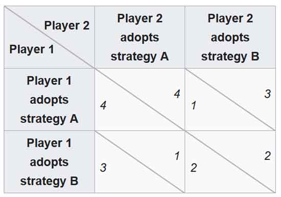
A sample coordination game showing relative payoff for player 1 (row) / player 2 (column) with each combination

The coordination game is a classic (symmetric) two player, two strategy game, with an example payoff matrix shown to the right. The players should thus coordinate, both adopting strategy A, to receive the highest payoff; i.e., 4. If both players chose strategy B though, there is still a Nash equilibrium. Although each player is awarded less than optimal payoff, neither player has incentive to change strategy due to a reduction in the immediate payoff (from 2 to 1).

A famous example of this type of game was called the stag hunt; in the game two players may choose to hunt a stag or a rabbit, the former providing more meat (4 utility units) than the latter (1 utility unit). The caveat is that the stag must be cooperatively hunted, so if one player attempts to hunt the stag, while the other hunts the rabbit, she/he will fail in hunting (0 utility units), whereas if they both hunt it they will split the payoff (2, 2). The game hence exhibits two equilibria at (stag, stag) and (rabbit, rabbit) and hence the players' optimal strategy depend on their expectation on what the other player may do. If one hunter trusts that the other will hunt the stag, they should hunt the stag; however if they suspect that the other will hunt the rabbit, they should hunt the rabbit. This game was used as an analogy for social cooperation, since much of the benefit that people gain in society depends upon people cooperating and implicitly trusting one another to act in a manner corresponding with cooperation.

Another example of a coordination game is the setting where two technologies are available to two firms with comparable products, and they have to elect a strategy to become the market standard. If both firms agree on the chosen technology, high sales are expected for both firms. If the firms do not agree on the standard technology, few sales result. Both strategies are Nash equilibria of the game.

Driving on a road against an oncoming car, and having to choose either to swerve on the left or to swerve on the right of the road, is also a coordination game. For example, with payoffs 10 meaning no crash and 0 meaning a crash, the coordination game can be defined with the following payoff matrix:

The driving game

In this case there are two pure-strategy Nash equilibria, when both choose to either drive on the left or on the right. If we admit mixed strategies (where a pure strategy is chosen at random, subject to some fixed probability), then there are three Nash equilibria for the same case: two we have seen from the pure-strategy form, where the probabilities are (0%, 100%) for player one, (0%, 100%) for player two; and (100%, 0%) for player one, (100%, 0%) for player two respectively. We add another where the probabilities for each player are (50%, 50%).
Prisoner's dilemma
Main article: Prisoner's dilemma

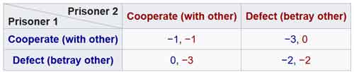
Example PD payoff matrix

Imagine two prisoners held in separate cells, interrogated simultaneously, and offered deals (lighter jail sentences) for betraying their fellow criminal. They can "cooperate" (with the other prisoner) by not snitching, or "defect" by betraying the other. However, there is a catch; if both players defect, then they both serve a longer sentence than if neither said anything. Lower jail sentences are interpreted as higher payoffs (shown in the table).

The prisoner's dilemma has a similar matrix as depicted for the coordination game, but the maximum reward for each player (in this case, a minimum loss of 0) is obtained only when the players' decisions are different. Each player improves their own situation by switching from "cooperating" to "defecting", given knowledge that the other player's best decision is to "defect". The prisoner's dilemma thus has a single Nash equilibrium: both players choosing to defect.

What has long made this an interesting case to study is the fact that this scenario is globally inferior to "both cooperating". That is, both players would be better off if they both chose to "cooperate" instead of both choosing to defect. However, each player could improve their own situation by breaking the mutual cooperation, no matter how the other player possibly (or certainly) changes their decision.

Network traffic
See also: Braess's paradox

Sample network graph. Values on edges are the travel time experienced by a 'car' traveling down that edge. x is the number of cars traveling via that edge.

An application of Nash equilibria is in determining the expected flow of traffic in a network. Consider the graph on the right. If we assume that there are x "cars" traveling from A to D, what is the expected distribution of traffic in the network?

This situation can be modeled as a "game" where every traveler has a choice of 3 strategies, where each strategy is a route from A to D (either ABD, ABCD, or ACD). The "payoff" of each strategy is the travel time of each route. In the graph on the right, a car travelling via ABD experiences travel time of (1+x/100)+2, where x is the number of cars traveling on edge AB. Thus, payoffs for any given strategy depend on the choices of the other players, as is usual. However, the goal, in this case, is to minimize travel time, not maximize it. Equilibrium will occur when the time on all paths is exactly the same. When that happens, no single driver has any incentive to switch routes, since it can only add to their travel time. For the graph on the right, if, for example, 100 cars are travelling from A to D, then equilibrium will occur when 25 drivers travel via ABD, 50 via ABCD, and 25 via ACD. Every driver now has a total travel time of 3.75 (to see this, note that a total of 75 cars take the AB edge, and likewise, 75 cars take the CD edge).

Notice that this distribution is not, actually, socially optimal. If the 100 cars agreed that 50 travel via ABD and the other 50 through ACD, then travel time for any single car would actually be 3.5, which is less than 3.75. This is also the Nash equilibrium if the path between B and C is removed, which means that adding another possible route can decrease the efficiency of the system, a phenomenon known as Braess's paradox.

Competition game

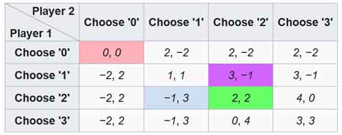
A competition game

This can be illustrated by a two-player game in which both players simultaneously choose an integer from 0 to 3 and they both win the smaller of the two numbers in points. In addition, if one player chooses a larger number than the other, then they have to give up two points to the other.

This game has a unique pure-strategy Nash equilibrium: both players choosing 0 (highlighted in light red). Any other strategy can be improved by a player switching their number to one less than that of the other player. In the adjacent table, if the game begins at the green square, it is in player 1's interest to move to the purple square and it is in player 2's interest to move to the blue square. Although it would not fit the definition of a competition game, if the game is modified so that the two players win the named amount if they both choose the same number, and otherwise win nothing, then there are 4 Nash equilibria: (0,0), (1,1), (2,2), and (3,3).
Nash equilibria in a payoff matrix

There is an easy numerical way to identify Nash equilibria on a payoff matrix. It is especially helpful in two-person games where players have more than two strategies. In this case formal analysis may become too long. This rule does not apply to the case where mixed (stochastic) strategies are of interest. The rule goes as follows: if the first payoff number, in the payoff pair of the cell, is the maximum of the column of the cell and if the second number is the maximum of the row of the cell - then the cell represents a Nash equilibrium.

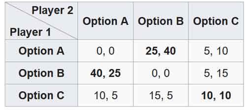
A payoff matrix – Nash equilibria in bold

We can apply this rule to a 3×3 matrix:

Using the rule, we can very quickly (much faster than with formal analysis) see that the Nash equilibria cells are (B,A), (A,B), and (C,C). Indeed, for cell (B,A) 40 is the maximum of the first column and 25 is the maximum of the second row. For (A,B) 25 is the maximum of the second column and 40 is the maximum of the first row. Same for cell (C,C). For other cells, either one or both of the duplet members are not the maximum of the corresponding rows and columns.

This said, the actual mechanics of finding equilibrium cells is obvious: find the maximum of a column and check if the second member of the pair is the maximum of the row. If these conditions are met, the cell represents a Nash equilibrium. Check all columns this way to find all NE cells. An N×N matrix may have between 0 and N×N pure-strategy Nash equilibria.
Stability

The concept of stability, useful in the analysis of many kinds of equilibria, can also be applied to Nash equilibria.

A Nash equilibrium for a mixed-strategy game is stable if a small change (specifically, an infinitesimal change) in probabilities for one player leads to a situation where two conditions hold:

the player who did not change has no better strategy in the new circumstance
the player who did change is now playing with a strictly worse strategy.

If these cases are both met, then a player with the small change in their mixed strategy will return immediately to the Nash equilibrium. The equilibrium is said to be stable. If condition one does not hold then the equilibrium is unstable. If only condition one holds then there are likely to be an infinite number of optimal strategies for the player who changed.

In the "driving game" example above there are both stable and unstable equilibria. The equilibria involving mixed strategies with 100% probabilities are stable. If either player changes their probabilities slightly, they will be both at a disadvantage, and their opponent will have no reason to change their strategy in turn. The (50%,50%) equilibrium is unstable. If either player changes their probabilities (which would neither benefit or damage the expectation of the player who did the change, if the other player's mixed strategy is still (50%,50%)), then the other player immediately has a better strategy at either (0%, 100%) or (100%, 0%).

Stability is crucial in practical applications of Nash equilibria, since the mixed strategy of each player is not perfectly known, but has to be inferred from statistical distribution of their actions in the game. In this case unstable equilibria are very unlikely to arise in practice, since any minute change in the proportions of each strategy seen will lead to a change in strategy and the breakdown of the equilibrium.

The Nash equilibrium defines stability only in terms of unilateral deviations. In cooperative games such a concept is not convincing enough. Strong Nash equilibrium allows for deviations by every conceivable coalition.[16] Formally, a strong Nash equilibrium is a Nash equilibrium in which no coalition, taking the actions of its complements as given, can cooperatively deviate in a way that benefits all of its members.[17] However, the strong Nash concept is sometimes perceived as too "strong" in that the environment allows for unlimited private communication. In fact, strong Nash equilibrium has to be Pareto efficient. As a result of these requirements, strong Nash is too rare to be useful in many branches of game theory. However, in games such as elections with many more players than possible outcomes, it can be more common than a stable equilibrium.

A refined Nash equilibrium known as coalition-proof Nash equilibrium (CPNE)[16] occurs when players cannot do better even if they are allowed to communicate and make "self-enforcing" agreement to deviate. Every correlated strategy supported by iterated strict dominance and on the Pareto frontier is a CPNE.[18] Further, it is possible for a game to have a Nash equilibrium that is resilient against coalitions less than a specified size, k. CPNE is related to the theory of the core.

Finally in the eighties, building with great depth on such ideas Mertens-stable equilibria were introduced as a solution concept. Mertens stable equilibria satisfy both forward induction and backward induction. In a game theory context stable equilibria now usually refer to Mertens stable equilibria.

Occurrence

If a game has a unique Nash equilibrium and is played among players under certain conditions, then the NE strategy set will be adopted. Sufficient conditions to guarantee that the Nash equilibrium is played are:

The players all will do their utmost to maximize their expected payoff as described by the game.
The players are flawless in execution.
The players have sufficient intelligence to deduce the solution.
The players know the planned equilibrium strategy of all of the other players.
The players believe that a deviation in their own strategy will not cause deviations by any other players.
There is common knowledge that all players meet these conditions, including this one. So, not only must each player know the other players meet the conditions, but also they must know that they all know that they meet them, and know that they know that they know that they meet them, and so on.

Where the conditions are not met

Examples of game theory problems in which these conditions are not met:

The first condition is not met if the game does not correctly describe the quantities a player wishes to maximize. In this case there is no particular reason for that player to adopt an equilibrium strategy. For instance, the prisoner's dilemma is not a dilemma if either player is happy to be jailed indefinitely.
Intentional or accidental imperfection in execution. For example, a computer capable of flawless logical play facing a second flawless computer will result in equilibrium. Introduction of imperfection will lead to its disruption either through loss to the player who makes the mistake, or through negation of the common knowledge criterion leading to possible victory for the player. (An example would be a player suddenly putting the car into reverse in the game of chicken, ensuring a no-loss no-win scenario).
In many cases, the third condition is not met because, even though the equilibrium must exist, it is unknown due to the complexity of the game, for instance in Chinese chess.[19] Or, if known, it may not be known to all players, as when playing tic-tac-toe with a small child who desperately wants to win (meeting the other criteria).

The criterion of common knowledge may not be met even if all players do, in fact, meet all the other criteria. Players wrongly distrusting each other's rationality may adopt counter-strategies to expected irrational play on their opponents’ behalf. This is a major consideration in "chicken" or an arms race, for example.

Where the conditions are met

In his Ph.D. dissertation, John Nash proposed two interpretations of his equilibrium concept, with the objective of showing how equilibrium points

(...) can be connected with observable phenomenon. One interpretation is rationalistic: if we assume that players are rational, know the full structure of the game, the game is played just once, and there is just one Nash equilibrium, then players will play according to that equilibrium. This idea was formalized by Aumann, R. and A. Brandenburger, 1995, Epistemic Conditions for Nash Equilibrium, Econometrica, 63, 1161-1180 who interpreted each player's mixed strategy as a conjecture about the behaviour of other players and have shown that if the game and the rationality of players is mutually known and these conjectures are commonly know, then the conjectures must be a Nash equilibrium (a common prior assumption is needed for this result in general, but not in the case of two players. In this case, the conjectures need only be mutually known).

A second interpretation, that Nash referred to by the mass action interpretation, is less demanding on players:

[i]t is unnecessary to assume that the participants have full knowledge of the total structure of the game, or the ability and inclination to go through any complex reasoning processes. What is assumed is that there is a population of participants for each position in the game, which will be played throughout time by participants drawn at random from the different populations. If there is a stable average frequency with which each pure strategy is employed by the average member of the appropriate population, then this stable average frequency constitutes a mixed strategy Nash equilibrium.

For a formal result along these lines, see Kuhn, H. and et al., 1996, "The Work of John Nash in Game Theory," Journal of Economic Theory, 69, 153–185.

Due to the limited conditions in which NE can actually be observed, they are rarely treated as a guide to day-to-day behaviour, or observed in practice in human negotiations. However, as a theoretical concept in economics and evolutionary biology, the NE has explanatory power. The payoff in economics is utility (or sometimes money), and in evolutionary biology is gene transmission; both are the fundamental bottom line of survival. Researchers who apply games theory in these fields claim that strategies failing to maximize these for whatever reason will be competed out of the market or environment, which are ascribed the ability to test all strategies. This conclusion is drawn from the "stability" theory above. In these situations the assumption that the strategy observed is actually a NE has often been borne out by research.[20]
NE and non-credible threats

Extensive and Normal form illustrations that show the difference between SPNE and other NE. The blue equilibrium is not subgame perfect because player two makes a non-credible threat at 2(2) to be unkind (U).

The Nash equilibrium is a superset of the subgame perfect Nash equilibrium. The subgame perfect equilibrium in addition to the Nash equilibrium requires that the strategy also is a Nash equilibrium in every subgame of that game. This eliminates all non-credible threats, that is, strategies that contain non-rational moves in order to make the counter-player change their strategy.

The image to the right shows a simple sequential game that illustrates the issue with subgame imperfect Nash equilibria. In this game player one chooses left(L) or right(R), which is followed by player two being called upon to be kind (K) or unkind (U) to player one, However, player two only stands to gain from being unkind if player one goes left. If player one goes right the rational player two would de facto be kind to her/him in that subgame. However, The non-credible threat of being unkind at 2(2) is still part of the blue (L, (U,U)) Nash equilibrium. Therefore, if rational behavior can be expected by both parties the subgame perfect Nash equilibrium may be a more meaningful solution concept when such dynamic inconsistencies arise.

Proof of existence
Proof using the Kakutani fixed-point theorem

Nash's original proof (in his thesis) used Brouwer's fixed-point theorem (e.g., see below for a variant). We give a simpler proof via the Kakutani fixed-point theorem, following Nash's 1950 paper (he credits David Gale with the observation that such a simplification is possible).

To prove the existence of a Nash equilibrium, let \( r_{i}(\sigma _{-i}) \) be the best response of player i to the strategies of all other players.

\( {\displaystyle r_{i}(\sigma _{-i})=\mathop {\underset {\sigma _{i}}{\operatorname {arg\,max} }} u_{i}(\sigma _{i},\sigma _{-i})} \)

Here, \( \sigma \in \Sigma \) , where \( \Sigma =\Sigma _{i}\times \Sigma _{-i} \), is a mixed-strategy profile in the set of all mixed strategies and \( u_{i}\) is the payoff function for player i. Define a set-valued function \( r\colon \Sigma \rightarrow 2^{\Sigma } \) such that \( {\displaystyle r=r_{i}(\sigma _{-i})\times r_{-i}(\sigma _{i})} \) . The existence of a Nash equilibrium is equivalent to r having a fixed point.

Kakutani's fixed point theorem guarantees the existence of a fixed point if the following four conditions are satisfied.

\( \Sigma \) is compact, convex, and nonempty.
\( r(\sigma ) \) is nonempty.
\( r(\sigma ) \) is upper hemicontinuous
\( r(\sigma ) \)is convex.

Condition 1. is satisfied from the fact that \( \Sigma \) is a simplex and thus compact. Convexity follows from players' ability to mix strategies. \( \Sigma \) is nonempty as long as players have strategies.

Condition 2. and 3. are satisfied by way of Berge's maximum theorem. Because \( u_{i} \) is continuous and compact, \( r(\sigma _{i}) \) is non-empty and upper hemicontinuous.

Condition 4. is satisfied as a result of mixed strategies. Suppose \( \sigma _{i},\sigma '_{i}\in r(\sigma _{-i}), \) then \( \lambda \sigma _{i}+(1-\lambda )\sigma '_{i}\in r(\sigma _{-i}) \) . i.e. if two strategies maximize payoffs, then a mix between the two strategies will yield the same payoff.

Therefore, there exists a fixed point in r {\displaystyle r} r and a Nash equilibrium.[21]

When Nash made this point to John von Neumann in 1949, von Neumann famously dismissed it with the words, "That's trivial, you know. That's just a fixed-point theorem." (See Nasar, 1998, p. 94.)

Alternate proof using the Brouwer fixed-point theorem

We have a game G=(N,A,u) where N is the number of players and \( {\displaystyle A=A_{1}\times \cdots \times A_{N}} \) is the action set for the players. All of the action sets \( A_{i \) } are finite. Let \( {\displaystyle \Delta =\Delta _{1}\times \cdots \times \Delta _{N}} \) denote the set of mixed strategies for the players. The finiteness of the \( A_{i} \)s ensures the compactness of \( \Delta \) .

We can now define the gain functions. For a mixed strategy \( \sigma \in \Delta \) , we let the gain for player i {\displaystyle i} i on action \( a\in A_{i} \) be

\( \displaystyle {\text{Gain}}_{i}(\sigma ,a)=\max\{0,u_{i}(a,\sigma _{-i})-u_{i}(\sigma _{i},\sigma _{-i})\}.}

The gain function represents the benefit a player gets by unilaterally changing their strategy. We now define \( g=(g_{1},\dotsc ,g_{N}) \) where

\( g_{i}(\sigma )(a)=\sigma _{i}(a)+{\text{Gain}}_{i}(\sigma ,a) \)

for \( \sigma \in \Delta ,a\in A_{i} \) . We see that

\( {\displaystyle \sum _{a\in A_{i}}g_{i}(\sigma )(a)=\sum _{a\in A_{i}}\sigma _{i}(a)+{\text{Gain}}_{i}(\sigma ,a)=1+\sum _{a\in A_{i}}{\text{Gain}}_{i}(\sigma ,a)>0.} \)

Next we define:

\( {\displaystyle {\begin{cases}f=(f_{1},\cdots ,f_{N}):\Delta \to \Delta \\f_{i}(\sigma )(a)={\frac {g_{i}(\sigma )(a)}{\sum _{b\in A_{i}}g_{i}(\sigma )(b)}}&a\in A_{i}\end{cases}}} \)

It is easy to see that each \( f_{i} \) is a valid mixed strategy in \( \Delta _{i} \). It is also easy to check that each \( f_{i} \) is a continuous function of σ {\displaystyle \sigma } \sigma , and hence f is a continuous function. As the cross product of a finite number of compact convex sets, \( \Delta \) is also compact and convex. Applying the Brouwer fixed point theorem to f and \( \Delta \) we conclude that f has a fixed point in\( \Delta \), call it \( \sigma ^{*} \). We claim that \( \sigma ^{*} \) is a Nash equilibrium in G. For this purpose, it suffices to show that

\( {\displaystyle \forall i\in \{1,\cdots ,N\},\forall a\in A_{i}:\quad {\text{Gain}}_{i}(\sigma ^{*},a)=0.} \)

This simply states that each player gains no benefit by unilaterally changing their strategy, which is exactly the necessary condition for a Nash equilibrium.

Now assume that the gains are not all zero. Therefore, \( {\displaystyle \exists i\in \{1,\cdots ,N\},} \) and \( a\in A_{i} \) such that\( {\text{Gain}}_{i}(\sigma ^{*},a)>0 \). Note then that

\( {\displaystyle \sum _{a\in A_{i}}g_{i}(\sigma ^{*},a)=1+\sum _{a\in A_{i}}{\text{Gain}}_{i}(\sigma ^{*},a)>1.} \)

So let

\( C=\sum _{{a\in A_{i}}}g_{i}(\sigma ^{*},a). \)

Also we shall denote \( {\text{Gain}}(i,\cdot ) \) as the gain vector indexed by actions in \( } A_{i} \). Since \( \sigma ^{*} \) is the fixed point we have:

\( {\displaystyle {\begin{aligned}\sigma ^{*}=f(\sigma ^{*})&\Rightarrow \sigma _{i}^{*}=f_{i}(\sigma ^{*})\\&\Rightarrow \sigma _{i}^{*}={\frac {g_{i}(\sigma ^{*})}{\sum _{a\in A_{i}}g_{i}(\sigma ^{*})(a)}}\\[6pt]&\Rightarrow \sigma _{i}^{*}={\frac {1}{C}}\left(\sigma _{i}^{*}+{\text{Gain}}_{i}(\sigma ^{*},\cdot )\right)\\[6pt]&\Rightarrow C\sigma _{i}^{*}=\sigma _{i}^{*}+{\text{Gain}}_{i}(\sigma ^{*},\cdot )\\&\Rightarrow \left(C-1\right)\sigma _{i}^{*}={\text{Gain}}_{i}(\sigma ^{*},\cdot )\\&\Rightarrow \sigma _{i}^{*}=\left({\frac {1}{C-1}}\right){\text{Gain}}_{i}(\sigma ^{*},\cdot ).\end{aligned}}} \)

Since C>1 we have that\( \sigma _{i}^{*} \) is some positive scaling of the vector \( {\text{Gain}}_{i}(\sigma ^{*},\cdot ) \). Now we claim that

\( {\displaystyle \forall a\in A_{i}:\quad \sigma _{i}^{*}(a)(u_{i}(a_{i},\sigma _{-i}^{*})-u_{i}(\sigma _{i}^{*},\sigma _{-i}^{*}))=\sigma _{i}^{*}(a){\text{Gain}}_{i}(\sigma ^{*},a)} \)

To see this, we first note that if \( {\text{Gain}}_{i}(\sigma ^{*},a)>0 \) then this is true by definition of the gain function. Now assume that \( {\text{Gain}}_{i}(\sigma ^{*},a)=0 \). By our previous statements we have that

\( {\displaystyle \sigma _{i}^{*}(a)=\left({\frac {1}{C-1}}\right){\text{Gain}}_{i}(\sigma ^{*},a)=0} \)

and so the left term is zero, giving us that the entire expression is 0 {\displaystyle 0} {\displaystyle 0} as needed.

So we finally have that

\( {\displaystyle {\begin{aligned}0&=u_{i}(\sigma _{i}^{*},\sigma _{-i}^{*})-u_{i}(\sigma _{i}^{*},\sigma _{-i}^{*})\\&=\left(\sum _{a\in A_{i}}\sigma _{i}^{*}(a)u_{i}(a_{i},\sigma _{-i}^{*})\right)-u_{i}(\sigma _{i}^{*},\sigma _{-i}^{*})\\&=\sum _{a\in A_{i}}\sigma _{i}^{*}(a)(u_{i}(a_{i},\sigma _{-i}^{*})-u_{i}(\sigma _{i}^{*},\sigma _{-i}^{*}))\\&=\sum _{a\in A_{i}}\sigma _{i}^{*}(a){\text{Gain}}_{i}(\sigma ^{*},a)&&{\text{ by the previous statements }}\\&=\sum _{a\in A_{i}}\left(C-1\right)\sigma _{i}^{*}(a)^{2}>0\end{aligned}}} \)

where the last inequality follows since \( \sigma _{i}^{*} \) is a non-zero vector. But this is a clear contradiction, so all the gains must indeed be zero. Therefore,\( \sigma ^{*} \) is a Nash equilibrium for G as needed.

Computing Nash equilibria

If a player A has a dominant strategy \( s_{A} \) then there exists a Nash equilibrium in which A plays \( s_{A} \). In the case of two players A and B, there exists a Nash equilibrium in which A plays \( s_{A} \) and B plays a best response to \( s_{A} \). If \( s_{A} \) is a strictly dominant strategy, A plays \( s_{A} \) in all Nash equilibria. If both A and B have strictly dominant strategies, there exists a unique Nash equilibrium in which each plays their strictly dominant strategy.

In games with mixed-strategy Nash equilibria, the probability of a player choosing any particular (so pure) strategy can be computed by assigning a variable to each strategy that represents a fixed probability for choosing that strategy. In order for a player to be willing to randomize, their expected payoff for each (pure) strategy should be the same. In addition, the sum of the probabilities for each strategy of a particular player should be 1. This creates a system of equations from which the probabilities of choosing each strategy can be derived.[13]

Examples

Matching pennies

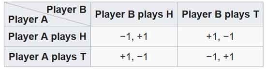
In the matching pennies game, player A loses a point to B if A and B play the same strategy and wins a point from B if they play different strategies. To compute the mixed-strategy Nash equilibrium, assign A the probability p of playing H and (1−p) of playing T, and assign B the probability q of playing H and (1−q) of playing T.

E[payoff for A playing H] = (−1)q + (+1)(1−q) = 1−2q
E[payoff for A playing T] = (+1)q + (−1)(1−q) = 2q−1
E[payoff for A playing H] = E[payoff for A playing T] ⇒ 1−2q = 2q−1 ⇒ q = 1/2

E[payoff for B playing H] = (+1)p + (−1)(1−p) = 2p−1
E[payoff for B playing T] = (−1)p + (+1)(1−p) = 1−2p
E[payoff for B playing H] = E[payoff for B playing T] ⇒ 2p−1 = 1−2p ⇒ p = 1/2

Thus a mixed-strategy Nash equilibrium, in this game, is for each player to randomly choose H or T with p = 1/2 and q = 1/2.

References

Game theory textbooks
Dixit, Avinash, Susan Skeath and David Reiley. Games of Strategy. W.W. Norton & Company. (Third edition in 2009)
Dutta, Prajit K. (1999), Strategies and games: theory and practice, MIT Press, ISBN 978-0-262-04169-0. Suitable for undergraduate and business students.
Fudenberg, Drew and Jean Tirole (1991) Game Theory MIT Press.
Leyton-Brown, Kevin; Shoham, Yoav (2008), Essentials of Game Theory: A Concise, Multidisciplinary Introduction, San Rafael, CA: Morgan & Claypool Publishers, ISBN 978-1-59829-593-1. An 88-page mathematical introduction; see Chapter 2. Free online at many universities.
Morgenstern, Oskar and John von Neumann (1947) The Theory of Games and Economic Behavior Princeton University Press
Myerson, Roger B. (1997), Game theory: analysis of conflict, Harvard University Press, ISBN 978-0-674-34116-6
Papayoanou, Paul (2010), Game Theory for Business: A Primer in Strategic Gaming, Probabilistic Publishing, ISBN 978-0964793873
Rubinstein, Ariel; Osborne, Martin J. (1994), A course in game theory, MIT Press, ISBN 978-0-262-65040-3. A modern introduction at the graduate level.
Shoham, Yoav; Leyton-Brown, Kevin (2009), Multiagent Systems: Algorithmic, Game-Theoretic, and Logical Foundations, New York: Cambridge University Press, ISBN 978-0-521-89943-7. A comprehensive reference from a computational perspective; see Chapter 3. Downloadable free online.
Gibbons, Robert (1992), Game Theory for Applied Economists, Princeton University Press (July 13, 1992), ISBN 978-0-691-00395-5. Lucid and detailed introduction to game theory in an explicitly economic context.
Osborne, Martin (2004), An introduction to game theory, Oxford University Press, ISBN 978-0-19-512895-6. Introduction to Nash equilibrium.
Binmore, Ken (2007), Playing for Real: A Text on Game Theory, Oxford University Press, ISBN 978-0195300574.
Original Nash papers
Nash, John (1950) "Equilibrium points in n-person games" Proceedings of the National Academy of Sciences 36(1):48-49.
Nash, John (1951) "Non-Cooperative Games" The Annals of Mathematics 54(2):286-295.
Other references
Mehlmann, A. (2000) The Game's Afoot! Game Theory in Myth and Paradox, American Mathematical Society.
Nasar, Sylvia (1998), A Beautiful Mind, Simon & Schuster.
Undergraduate Texts in Mathematics
Graduate Studies in Mathematics
Hellenica World - Scientific Library
Retrieved from "http://en.wikipedia.org/"
All text is available under the terms of the GNU Free Documentation License